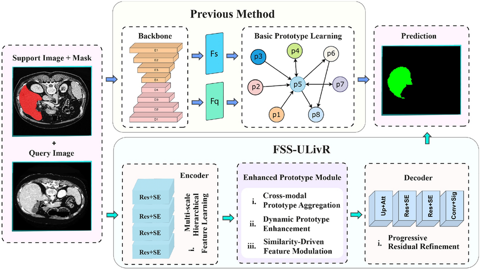
This section details the architecture and components of our proposed FSS-ULivR model for few-shot liver segmentation. The model integrates a ResNet-based encoder with an enhanced prototype module that integrates a transformer block for global feature representation and an SE block for dynamic channel-wise refinement (Raiaan et al. 2024). In the decoder, attention gates are applied to effectively handle the challenges posed by limited annotated data (Rahman et al. 2022; Ouyang et al. 2022; Abian et al. 2024). Figure 2 demonstrates the overall structure of the FSS-ULivR model.

Few-shot learning strategy

In our FSS-ULivR framework, our training follows a 1-shot episodic setup, where each episode provides exactly one support image–mask pair \((I_s, M_s)\) and a single query image \(I_q\). The objective is to utilize this minimal supervision to predict the query mask \(\hat_q\) (Zhang et al. 2021). To achieve this, we first project both support and query images into a shared feature space using a deep encoder E, as demonstrated in Equation (1):

$$\begin F_s, \\} = E(I_s), \quad F_q, \\} = E(I_q) \end$$

(1)

where \(F_* \in \mathbb ^\) denotes the bottleneck feature map and \(\\}\) are multi-scale feature maps used in skip connections. The encoder is composed of residual blocks, each incorporating a Squeeze-and-Excitation (SE) operation to recalibrate channel-wise activations. Next, we extract a refined prototype P from the support features using our Enhanced Prototype Module. After applying an SE block and a stack of transformer layers to \(F_s\), we resize \(M_s\) to match \(F_s\) spatially and compute the prototype in Equation (2):

$$\begin P = \frac F_s(i,j) \cdot M_s(i,j)} M_s(i,j) + \epsilon } \in \mathbb ^ \end$$

(2)

where \(\epsilon \) is a small constant for numerical stability. We then apply safe L2 normalization and a channel-attention head to enhance the discriminative capacity of P. To localize the same semantic class in the query image, we refine \(F_q\) through SE and transformer layers, and compute a similarity map by taking the dot-product between normalized query features and the prototype, which is expanded spatially to match the query features, as shown in Equation (3):

$$\begin S_q(i,j) = \frac_q(i,j), P \rangle }_q(i,j) \Vert \cdot \Vert P \Vert }, \quad S_q \in [0,1]^ \end$$

(3)

where \(\tilde_q\) denotes the normalized query feature map. The similarity map \( S_q \) emphasizes regions likely to belong to the target class, and we modulate the original query features \( F_q \) via element-wise multiplication of \(F_q\) and \(S_q\), which results in \(F_q'\). The decoder, which mirrors the encoder using upsampling layers, Improved Attention Gates for each skip-connection, and residual blocks, takes as input \(F_q'\) along with multi-scale skip features \(S_q^\) and reconstructs the output mask as demonstrated in Equation (4):

$$\begin \hat_q = \sigma \left( \text _ \left( D \left( \\} \right) \right) \right) \end$$

(4)

where \(D(\cdot )\) denotes the decoder module and \(\sigma \) is the sigmoid activation function that produces the final binary mask.

The training objective optimizes a hybrid loss function that balances overlap, class imbalance, and boundary alignment by combining Dice loss, Focal loss, Tversky loss, and Binary Cross-Entropy (BCE) loss. This composite loss enables the model to effectively learn accurate segmentation boundaries while handling imbalanced data. By sampling diverse episodes with varying anatomical structures, FSS-ULivR generalizes effectively from just a single annotated support example.

Encoder

Our encoder extracts high-level feature representations from both support and query images. It operates in two parallel branches (one for support and one for query) that share an identical architecture.

Each branch comprises multiple residual blocks enhanced with SE modules, and the features are progressively reduced by max pooling (Mahmud et al. 2021). This design preserves spatial hierarchies while maintaining rich feature representations that are crucial for subsequent fusion in the prototype module and refinement in the decoder.

Fig. 3

Illustration of the core components in the FSS-ULivR model: A. Residual Block, B. Squeeze-Excitation (SE) Block, C. Attention Gate, and D. Transformer Block, integrated for enhanced performance in few-shot segmentation

Residual blocks with SE modules

Residual blocks serve as the backbone of our encoder network. The input feature map \( F_} \in \mathbb ^ \) is processed through the residual block, where \( C \) represents the number of channels and \( H \times W \) denote the spatial dimensions. Each block contains a main path with SE module, skip connections, and the output derived from the residual block. The integrated SE modules help the block focus on important channels and improve feature learning across different spatial levels. Figure 3A illustrates the Residual Block of our FSS-ULivR model.

We compute the main path first by applying a \(3 \times 3\) convolution, then applying batch normalization and a Rectified Linear Unit (ReLU) activation as shown in Equation (5).

$$\begin F_1 = \operatorname \Bigl ( \gamma \bigl (W_1 * F_} + b_1\bigr ) \Bigr ) \end$$

(5)

where \(W_1\) is a \(3 \times 3\) kernel, \(b_1\) is the bias, \(\gamma \) denotes batch normalization, and \(*\) represents the convolution operation. Then, we perform a second \(3 \times 3\) convolution, after which batch normalization is applied in Equation (6).

$$\begin F_2 = \gamma \Bigl (W_2 * F_1 + b_2\Bigr ) \end$$

(6)

where \(W_2\) is another \(3 \times 3\) convolution kernel, and \(b_2\) is its corresponding bias term. Following Equation (6), we refine the channel-wise features using an SE module, which includes squeeze, excitation, and recalibration steps. This refinement explicitly models interdependencies between channels, enhancing the representation of discriminative spatial hierarchies. Figure 3B illustrates the SE Block of our FSS-ULivR model.

The squeeze operation aggregates spatial information by computing channel-wise statistics through Global Average Pooling (GAP) in Equation (7), which results in a vector \(z \in \mathbb ^\).

$$\begin z_c = \frac \sum _^ \sum _^ F_2(c,i,j), \quad c = 1, \ldots, C \end$$

(7)

The excitation operation then learns channel-specific scaling factors that capture the relative importance of each feature channel for the given spatial context. The vector \(z\) is passed through two fully connected layers to generate these scaling factors in Equation (8):

$$\begin s = \sigma \Bigl ( W_ \cdot \operatorname \bigl (W_ \cdot z + b_\bigr ) + b_ \Bigr ) \end$$

(8)

where \(W_ \in \mathbb ^ \times C}\) and \(W_ \in \mathbb ^}\) are weight matrices, \(b_\) and \(b_\) are biases, \(r\) is the reduction ratio, and \(\sigma \) refers to the sigmoid function. This two-stage fully connected architecture enables the SE module to learn complex, non-linear channel relationships while maintaining computational efficiency through dimensionality reduction. The recalibration step applies these learned scaling factors to selectively emphasize or suppress different channels based on their relevance to the current spatial context, as shown in Equation (9):

$$\begin F_2^}(c,i,j) = s_c \cdot F_2(c,i,j), \quad \forall \, c, i, j. \end$$

(9)

This channel-wise recalibration is particularly beneficial for few-shot segmentation as it helps the encoder focus on the most discriminative features while preserving spatial hierarchies across different resolution levels, while also providing an adaptive reweighting mechanism that makes the residual blocks sensitive to task-specific variations in the support-query pairs, which is critical in few-shot scenarios. To facilitate gradient flow, we further add a skip connection, \(F_\), and apply a \(1 \times 1\) convolution for dimension matching before addition. The \(F_\) is then passed as the input to the residual block \(F_\). The final output of the residual block \(F_}\) is then obtained by integrating the recalibrated main path (see Equation (9)) with the skip connection, followed by a ReLU activation. Finally, we apply max pooling to reduce the spatial dimensions after each residual block and to capture contextual information at multiple scales.

Parallel processing for support and query

In our experiment, we processed both support and query images using identical encoder branches. Then we stored the intermediate feature maps at different levels as skip connections. These features in the decoder are used to recover spatial details lost during downsampling.

Enhanced prototype module

Our Enhanced Prototype Module refines and fuses features from the support and query branches through two parallel processes. One processes support features to compute a robust prototype, while the other refines query features prior to fusion. The module utilizes transformer-based self-attention to capture global spatial dependencies and channel attention mechanisms to emphasize discriminative features, creating a unified approach that significantly improves support-query feature alignment in few-shot segmentation scenarios. In addition, we compute a cosine similarity map between the fused query features and the final support prototype by normalizing both along the channel dimension. This similarity map is then scaled to the range [0, 1] to form a spatial attention mask that guides the decoder.

Support processing stream

We first refine the support features using an SE block (as detailed in Equations (7)-(9)), ensuring that the most informative channels are emphasized. This channel-wise recalibration enhances the support features by emphasizing responses most relevant to the target class while suppressing background noise, which is particularly crucial when working with limited annotated examples. We then apply L2 normalization to these enhanced features before prototype pooling, ensuring that the subsequent similarity computation remains scale-invariant. We also refine the recalibrated support features utilizing transformer blocks as illustrated in Fig. 3D. The flattened support features are represented as \( X \in \mathbb ^ \), where \( N \) denotes the number of tokens and \( d \) refers to the feature dimension. We start the process by computing linear projections of query (Q), key (K), and value (V) for learnable parameter X. The transformer-based self-attention mechanism enables each spatial token in \( X \) to aggregate information from all other tokens, capturing global anatomical and contextual relationships that conventional convolutional operations fail to represent effectively. We use normalization to keep the prototype and query features on a similar scale, making the cosine similarity calculation more accurate. We then compute scaled dot-product attention in Equation (10), and calculate multi-head attention (MHA) subsequently in Equation (11):

$$\begin & \operatorname (Q, K, V) = \operatorname \left( \frac} \right) V \end$$

(10)

$$\begin & \operatorname (X) = \operatorname \bigl (\operatorname _1, \ldots, \operatorname _h\bigr ) W_O \end$$

(11)

where \(W_O \in \mathbb ^\) and \(h\) is the number of heads. We then apply a feed-forward network (FFN) with subsequent residual connections and layer normalization in Equation (12):

$$\begin \operatorname (x) = W_ \cdot \operatorname \Bigl (W_ \cdot x + b_\Bigr ) + b_ \end$$

(12)

The refined support features are then passed through the residual connection, followed by layer normalization in 2 steps. In the first step, we compute the output of the MHA, \(X'\), to the original input X. Then we applied layer normalization to this sum. In the second step, we add this to the output of the FFN, followed by second-layer normalization to generate \(X''\). The refined support features preserve both the original context and the newly captured dependencies. This global context modeling produces features that are robust to local variations in shape, size, or appearance, which is essential, particularly when only a few annotated examples are available for training. We then compute the support prototype using a binary support mask \(M \in \^\), which aggregates the features corresponding to the target class into a compact representation as demonstrated in Equation (13):

$$\begin P = \frac M(i,j) \cdot X''(i,j)} M(i,j) + \epsilon } \end$$

(13)

where \(\epsilon \) represents a minimal value to avoid division by zero. Here \(X''\) has already been L2-normalized in its channel dimension, so \(P\) inherits normalized scale. We further refine the prototype by applying a channel attention mechanism as shown in Equation (14):

$$\begin P_} = \sigma \Bigl ( W_} \cdot \operatorname \bigl (W_} \cdot P + b_}\bigr ) + b_} \Bigr ) \odot P \end$$

(14)

where \(\odot \) denotes the element-wise multiplication. This channel attention mechanism adaptively adjusts the prototype based on channel-wise relevance, producing a support prototype \( P_} \) that is both semantically rich from global context modeling and refined through attention-based weighting of feature channels.

Query processing stream

We first recalibrate the query features, denoted by \(X_}\), using an SE block, and then refine them by transformer blocks similar to those used in the support stream. The SE block enhances query features by emphasizing channels that correspond to the support prototype’s characteristics, while the transformer blocks provide each query location with global context, improving detection of target objects despite appearance variations. To ensure accurate comparison, we first L2-normalize the query feature vectors along the channel dimension so they match the scale of the support prototype before computing similarity. Specifically, we capture long-range dependencies in our query features by utilizing MHA, which is subsequently refined using FFN. The recalibrated query features, \(X_}'\), are computed after processing the first recalibrated features with an MHA followed by a normalization layer; it is then refined (denoted as \(X_}''\)) with an FFN followed by a second normalized layer. We then fuse the refined query features with the support prototype to refine the query features by utilizing information from the support set. To align the spatial dimensions, we broadcast the support prototype \(P\) to form \(\tilde\). Our fusion operation is defined in Equation (15):

$$\begin F_} = \operatorname \Bigl ( \gamma \Bigl (W_} * \operatorname \bigl (X_}'', \tilde\bigr ) + b_} \Bigr ) \Bigr ) \end$$

(15)

where \(\operatorname \) combines the query features with the broadcast support prototype. Then we compute a similarity map based on the fused features and the channel-modulated support prototype in Equation (16):

$$\begin S(i,j) = \frac}(i,j), P_} \rangle }}(i,j)\Vert \, \Vert P_}\Vert } \end$$

(16)

Both vectors are L2-normalized along the channel dimension, so \( S(i,j) \) ranges between \(-1\) and \(1\). We then scale it to the range \([0,1]\) using \(\frac\) and clip values to avoid numerical instability. We then refine the query features to construct modulated features \(F_\), using the similarity score, and scaling the fused features, \(F_\), based on their similarity to the support prototype, S(i, j). This similarity map acts as an attention mask, highlighting regions most similar to \(P_}\) and filtering out irrelevant areas. By integrating spatially global self-attention with channel-wise recalibration in both support and query streams, the Enhanced Prototype Module achieves precise and context-aware support-query feature alignment, thereby significantly boosting few-shot segmentation accuracy and robustness under limited annotation scenarios. The resulting \(F_}\) is then passed to the decoder, so that the following upsampling and fusion with skip connections focus on areas most likely to contain the target class.

Decoder

Our decoder reconstructs the segmentation map from the modulated query features by incorporating high-resolution details from the encoder’s skip connections, following a design with progressive upsampling, attention gating, and residual refinement (Li et al. 2024). The integration of improved attention gates and residual refinement blocks provides crucial advantages for restoring fine spatial details, particularly in recovering object boundaries and small-scale structures essential for accurate few-shot segmentation.

Upsampling and skip connections

At each decoding level \(l\), we upsample the modulated feature map \(F_}^\) to match the spatial dimensions of the corresponding encoder feature map \(F_}^\), as \(F_}^\), where each of the following modulated feature map is upsampled. We then concatenate the upsampled feature with the encoder feature. This concatenation \(F_^\) allows us to recover spatial details that were lost during downsampling.

Improved attention gates

We apply attention gates as illustrated in Fig. 3C to the skip connections to emphasize the most relevant features. These gates address the fundamental challenge of selective feature integration by dynamically weighting skip connections based on spatial and contextual relevance, effectively suppressing background noise while preserving target object boundaries. We then apply \(1 \times 1\) convolutions to the skip connection feature \(x\) and the gating signal \(g\) from the upsampled features, as described in Equation (17):

$$\begin \tilde = W_x * x + b_x, \quad \tilde = W_g * g + b_g. \end$$

(17)

We then fuse these two transformed features and apply a ReLU activation to generate the attention coefficients, as \(f\). Next, we compute the attention map \(\alpha \) using a \(1 \times 1\) convolution and then applying a sigmoid activation. We then modulate the skip connection (\(x_\)) by combining the initial skip connection feature x with the attention map \(\alpha \), which emphasizes the relevant spatial features to preserve fine-grained details while suppressing irrelevant ones.

Feature fusion and residual refinement

In this stage, we concatenate the modulated skip connection \(x_}\) with the upsampled feature map \(F_}^\) for creating the fused feature set \(F_}^\). This fused feature is then refined using additional residual blocks with SE modules, following the same formulation as described in Sect. 3.2.1. The residual refinement blocks help improve training by ensuring effective gradient flow and progressively enhancing features through channel-wise recalibration with SE modules. This process is crucial for recovering fine spatial details, as the SE modules adaptively emphasize important channels that capture object boundaries and small structures, while the residual connections preserve key spatial information throughout refinement. After the final refinement, we apply a convolutional layer to produce the segmentation logits as \(F_}\). Finally, we use a sigmoid activation function (\(\sigma \)) to convert the logits \(F_(i, j)\) into probabilities, which generates the final segmentation mask \(\hat(i,j)\). By selectively emphasizing relevant features and adaptively recalibrating channels, the attention gates and residual refinement blocks with SE modules enable precise restoration of fine details, which is crucial for accurate few-shot segmentation from limited data.

Loss functions

The FSS-ULivR model employs a composite loss function that integrates multiple loss metrics, including Dice loss, Focal loss, Tversky loss, and Binary Cross-Entropy (BCE) loss to improve segmentation accuracy and robustness. The Dice loss is derived from the Dice coefficient (see Sect. 4.2.1). The BCE loss, \( L_} \), is given by Equation (18):

$$\begin L_} = -\frac \sum _^N \left[ y_i \log \hat_i + (1 - y_i) \log (1 - \hat_i) \right] \end$$

(18)

where \( y_i \) and \( \hat_i \) represent the true label and predicted probability for the \( i \)-th pixel, respectively. The Focal loss, \( L_} \) as defined in Equation (19), addresses class imbalance by reducing the relative loss for well-classified examples and focusing more on hard, misclassified examples.

$$\begin \begin L_}&= - \frac \sum _^N \alpha \,(1 - p_i)^\gamma \bigl [\,y_i \log (p_i) \\&\qquad \quad + (1 - y_i)\log (1 - p_i)\bigr ] \end \end$$

(19)

where \( p_i = \hat_i \) is the predicted probability for class 1, \(\alpha \) is a weighting factor for balancing positive and negative examples, and \(\gamma \) is the focusing parameter that adjusts the rate at which easy examples are down-weighted. The Tversky loss, \( L_} \), is a generalization of the Dice loss that allows control over the penalty of false positives and false negatives as defined in Equation (20), which is useful for imbalanced datasets:

$$\begin L_} = 1 - \frac \end$$

(20)

where \(TP\), \(FN\), and \(FP\) denote true positives, false negatives, and false positives, respectively; \(\alpha \) and \(\beta \) control the penalties for false negatives and false positives; and \(\epsilon \) is a small constant to avoid division by zero. The final combined loss function, computed in Equation (21), is a weighted sum of these individual losses.

$$\begin L_} = \alpha \, L_} + \beta \, L_} + \gamma \, L_} + \delta \, L_} \end$$

(21)

where \(\alpha \), \(\beta \), \(\gamma \), and \(\delta \) are non-negative weighting coefficients balancing the contributions of each loss term, with their sum equal to one. This integrated loss formulation ensures both accurate pixel-level boundary delineation and effective handling of class imbalance, leading to improved segmentation performance. The values of these coefficients were empirically determined. Further details of this tuning process are discussed in Sect. 5.6.

Training procedure

Our training procedure consists of two stages: episodic few-shot segmentation training on the LiTS dataset, followed by cross-dataset validation on multiple external datasets.

In the first stage, we create 1-shot episodes by sampling a single support image–mask pair \((I_s, M_s)\) and a query image \(I_q\) from the LiTS training set. Each raw CT slice is first min–max normalized, resized to the target resolution, and windowed to highlight soft-tissue regions.

The processed support and query images are then passed through our ResNet-based encoder with SE blocks to extract multi-scale features. The Enhanced Prototype Module computes a refined support prototype and creates a similarity map, which is used to guide the query features during decoding. We train the model using a combined loss function composed of Dice loss, Focal loss, Tversky loss, and Binary Cross-Entropy (BCE) loss. The training employs the Adam optimizer with a fixed learning rate of 0.001, gradient clipping with a norm of 1.0, and a batch size of one episode. After completing N epochs of training, we freeze the model parameters and perform cross-dataset validation. For each external dataset \(D_i \in \, \text , \text ,\) MSD-Task03-Liver}, we prepare the data loader and normalization steps, then evaluate the trained model on all available images from that dataset.

We compute metrics such as Dice coefficient, specificity, and IoU to measure the model’s performance. No additional training or fine-tuning is applied during this evaluation; we directly test the trained model to show how well FSS-ULivR works on data with different characteristics and from different sources.

Algorithm 1 provides an overview of both the episodic training and the evaluation process. This two-stage approach ensures that our model not only learns from limited examples but also performs well on entirely new datasets without needing extra adjustments.

Algorithm 1

FSS-ULivR: Few-Shot Segmentation Workflow