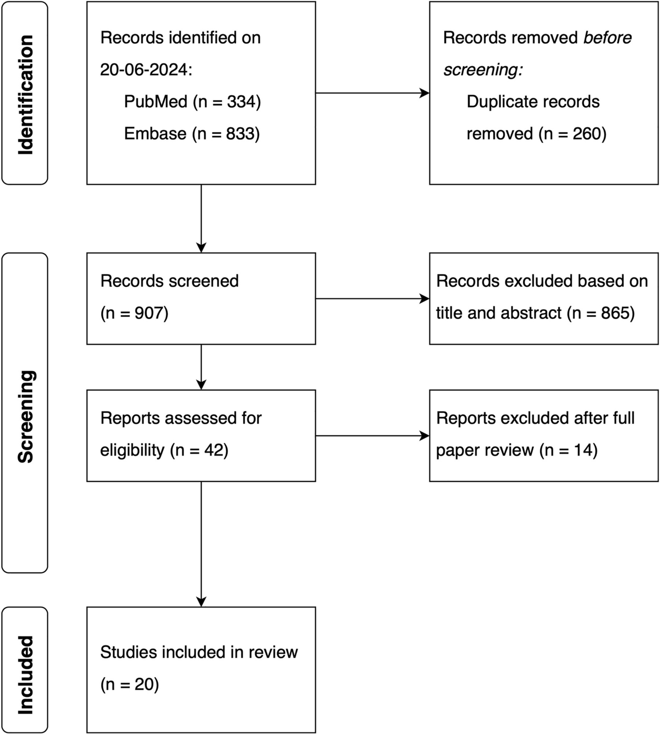
The data for this analysis originated from one phase 1 trial of healthy participants (HS-19–664, octreotide IR and CAM2029) and two phase 3 trials of patients with acromegaly (HS-18–633 and HS-19–647, CAM2029 only) where serial plasma collection was performed for all treatment groups. Trial designs, full eligibility criteria, sampling schedules and details of sample analysis for each trial can be found in Online Resource 1. Participants who completed trial HS-18–633 were able to continue onto trial HS-19–647, and these patients were treated as the same individual across trials in the analysis. Some participants had non-zero baseline levels of octreotide, as they were already on a stable dose of octreotide LAR or had continued on trial HS-19–647 from trial HS-18–633 and therefore were already receiving CAM2029.

Octreotide concentrations were analysed in plasma containing dipotassium ethylenediaminetetraacetic acid using a validated ultra-performance liquid chromatography method with tandem mass spectrometry detection, which was fully validated for precision, accuracy and reproducibility before application to the sample analysis. The lower limit of quantification (LOQ) was 0.0286 ng/mL. A similar method to that used in the current trials was used to collect observed octreotide LAR data by Tiberg et al., facilitating comparisons between their data and the data from this analysis [10].

This analysis included 4098 observations from 216 participants (further details can be found in Online Resource 2). In total, 75 healthy participants and 141 participants with acromegaly were included in the analysis; baseline characteristics of the participants in the PK analysis data set can be found in Table 1 and Online Resource 3. Overall, 3606 observations were from injections in the abdomen (88.0%), 422 were from injections in the thigh (10.3%), 60 were from injections in the buttock (1.5%) and the injection site was missing for 10 observations (0.2%). Ethics approval and the informed consent from each trial participant were obtained before trial inclusion, as detailed previously in the primary publications from the three clinical trials or within the appropriate records on the EudraCT or ClinicalTrials.gov registries (registration numbers: 2020–002643-35, NCT04076462, NCT04125836).

The population modelling analyses were performed using nonlinear mixed-effects modelling (NONMEM, version 7.5) installed on a computing cluster running Red Hat Enterprise Linux 8 [17]. Nonlinear mixed-effects modelling runs were performed using the GCC compiler, version 7.5, facilitated by Perl-speaks-NONMEM (PsN), version 5.2.6 [18, 19]. Data management and further processing of NONMEM output were performed using R version 3.5.3 (2019-03-11) [20, 21]. Parameter estimation was performed using the first-order conditional estimation method with interaction (FOCEI) method in NONMEM and the standard errors of the parameter estimates were computed using the MATRIX=S option in the NONMEM $COV record.

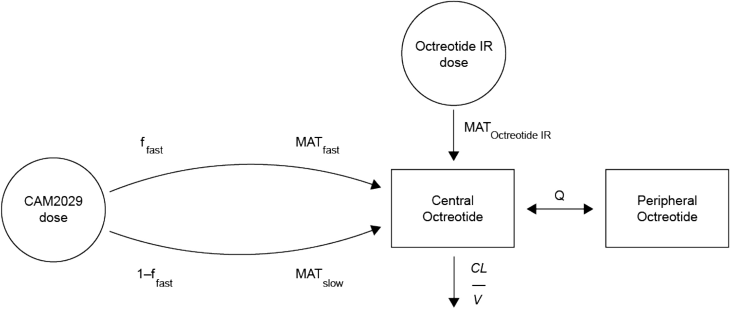
The model developed was a joint model for both CAM2029 and octreotide IR using log-transformed (natural logarithm) plasma concentrations. A one-compartment model with two different first-order absorption processes for CAM2029 and octreotide IR, and with first-order elimination, was the starting point for the model development. The starting model also included the mechanistic covariates defined in Table 2 and a parameter for bioavailability (F) with a fixed value of 1 for both CAM2029 and octreotide IR to facilitate the estimation of inter-individual variability (IIV) in the extent of absorption. A parameter (“fudge factor”) represented the octreotide PK concentration before the first CAM2029 dose was estimated in pre-treated participants with octreotide. Initially, all parameters in the model were associated with exponential IIVs to ensure that the individual PK parameters had a lower bound of zero, as shown in Eq. 1:

where TVPi is the typical parameter value for an individual, i, given the covariate values of this specific individual, Pi is the individual value of the parameter and \(\eta_ }}\) is a normally distributed random variable with mean 0 and standard deviation (SD) ωp. The variance-covariance matrix of the ωs is denoted Ω.

The starting residual unexplained variability (RUV) model was a proportional model with an exponential IIV term on the ϵ. With log-transformed data, the RUV model was implemented as additive on the log-scale (Eq. 2). The η on ϵ was included to manage between-individual variability in RUV and/or outliers.

$$\text(_)=\text\left(}_\right)+_,ij}\cdot ^_}$$

(2)

where yij is the jth observation for the ith individual, \(\hat_\) are the corresponding model predictions, often referred to as individual prediction, and ϵadd,ij is a normally distributed random variable, with mean 0 and with standard deviation and σadd.

Alternative structural models considered were two- and three-compartment models combined with zero- or first-order absorption processes (or combinations thereof), and terms/models that handled potential absorption delays. The discrimination between models was based mainly on inspection of graphical diagnostics and changes in objective function value (OFV) provided by NONMEM. A more complicated model was only retained if it provided a significant improvement (p < 0.05, − 3.84 change in OFV) and plausible parameter estimates that were not associated with excessively high relative standard errors (RSEs). Furthermore, it should preferably demonstrate improvements in the graphical diagnostics and not lead to a high (> 1000) condition number.

The base model, including the mechanistic covariates defined in Table 2, was used as a starting point for covariate analysis. The mechanistic covariates were those with a known impact on one or more parameters of the model such as body weight (WT) on clearance (CL) and volumes of distribution. For the mechanistic covariate of WT, the power relation was used (Eq. 3):

$$}_}_}}=}\right)}^_}}$$

(3)

The exploratory covariates, which were covariates that were not mechanistic, would not be expected to have an impact on one or more model parameters (structural covariates) and were explored for hypothesis-generating reasons, are presented in Table 2. Potential covariate-parameter relationships were evaluated using the stepwise covariate model-building procedure (SCM) with adaptive scope reduction and stage-wise filtering, which categorised covariates into the three aforementioned groups [22, 23]. The forward selection and backward elimination p values were 0.01 and 0.001, respectively. A strong correlation between population (patients with acromegaly or healthy participants) and age was found; age was chosen for inclusion in the covariate model due to its continuous nature. Body mass index (BMI) was tested on the absorption parameters rather than WT, as this was more appropriate for the SC route of administration. Continuous covariate-parameter relationships were implemented as exponential models (Eq. 4), while categorical covariate-parameter relationships were implemented as a fractional difference to the most common category (Eq. 5):

$$}_}_}=^_\cdot (\text-}_})}$$

(4)

$$}_}_}=\left\1\\ 1+_\end\genfrac=}_}}\ne _}}\right.$$

(5)

where θm is the covariate coefficient for covariate m, and Covm,ref is a reference covariate value for covariate m, to which the covariate model is normalised. For the mechanistic covariate of WT, the power relation was used (Eq.  3). The total effect of covariates on a parameter P was then calculated as the product of the n covariate terms in Eq. 6:

$$}_= _\cdot \prod_^}_}_}$$

(6)

where θp is the population typical parameter value (for an individual with typical/reference covariate values). The impact of covariates on selected secondary PK parameters (Cmax,ss and AUCτ,ss) was illustrated using forest plots [24]. The forest plots were generated using the final model and the uncertainty in the covariate effects was obtained by drawing 250 samples from a variance-covariance matrix computed from a non-parametric bootstrap with 30 samples.

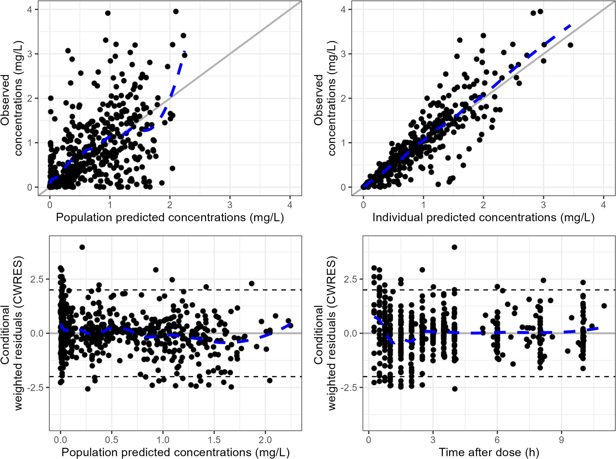
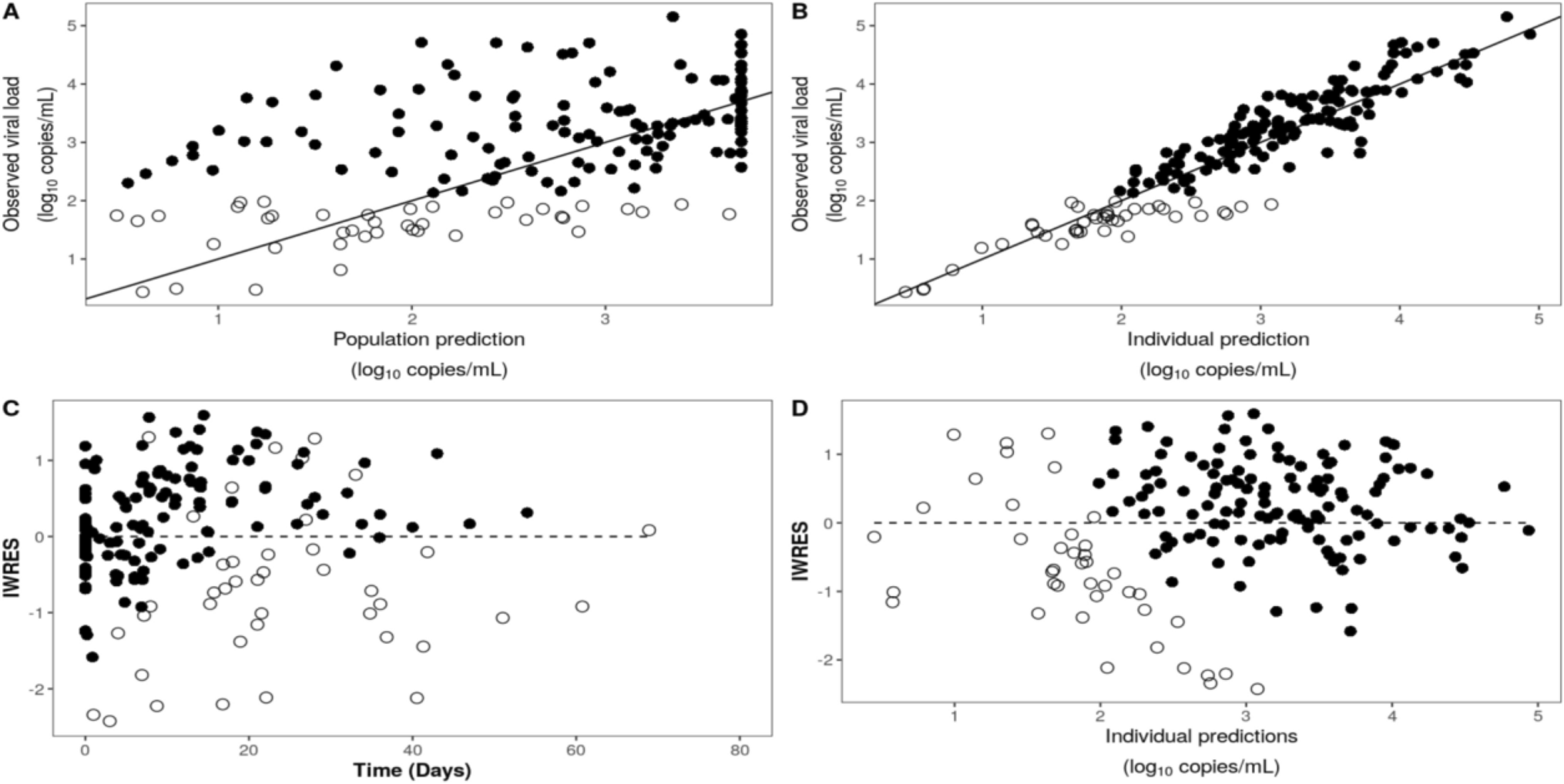
Model evaluation was based on the inspection of RSEs, plausibility of the parameter estimates, and graphical diagnostics, including goodness of fit (GOF) and visual predictive checks, as well as changes in the OFV provided by NONMEM. For GOF plots, plots of observations versus predictions were evaluated for random scatter around the line of identity, while conditional weighted residual (CWRES) plots were evaluated for random scatter around the zero line.

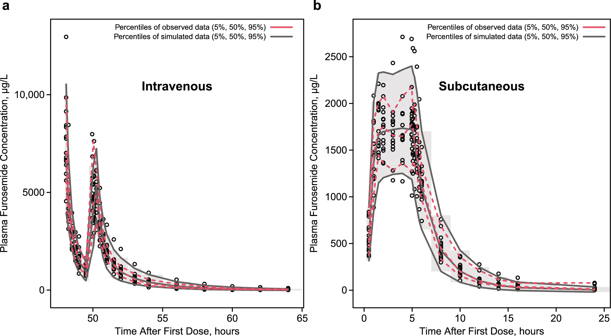
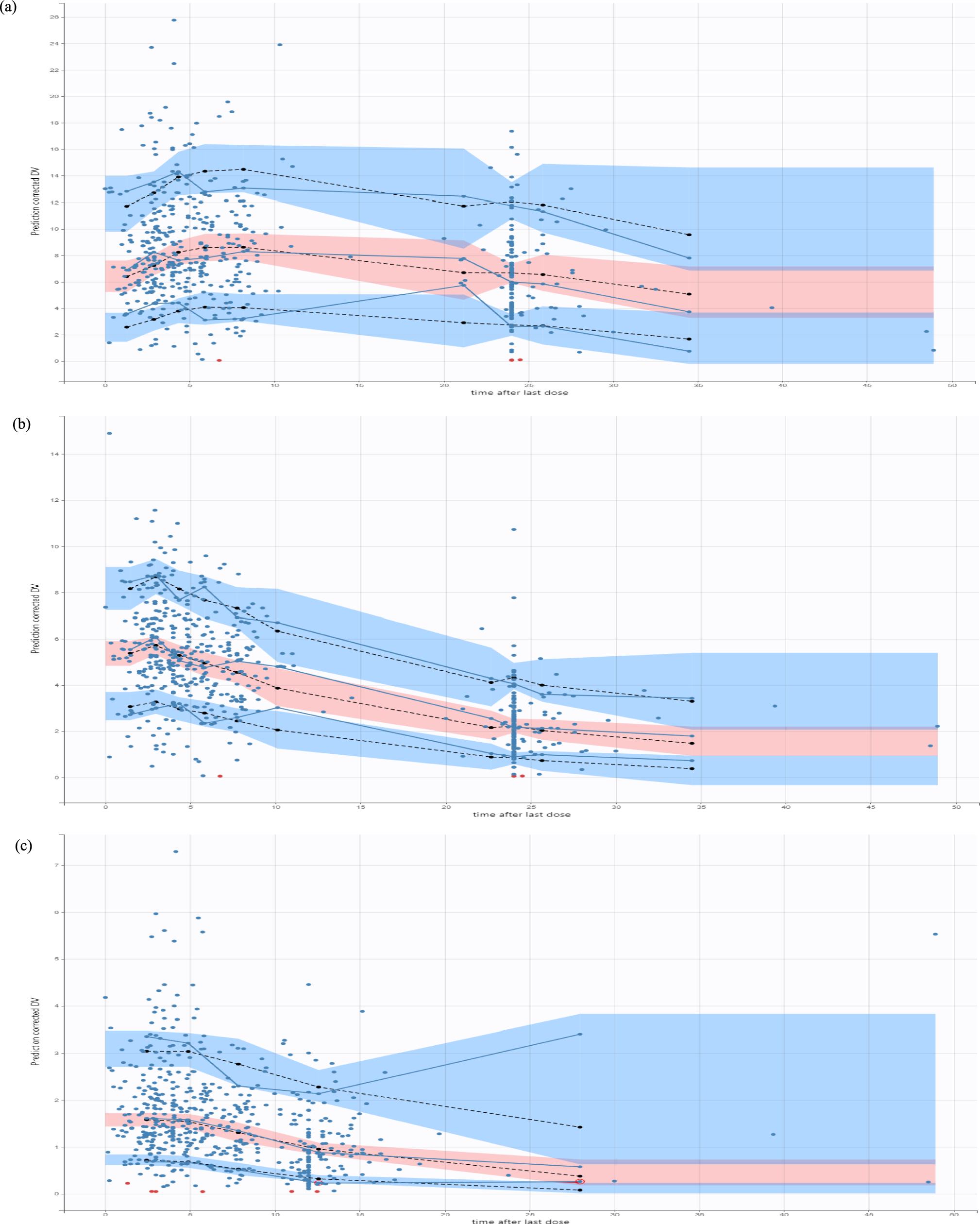
Prediction-corrected visual predictive checks (pcVPCs) were used to evaluate the predictive performance of the key models in the analysis [25, 26]. Data were simulated 200 times using the doses and covariate data from the participants in the analysis data set, using the same trial design. All observations in the analysis data set plus all below LOQ observations were included in the visual predictive checks (VPC) analyses, and the LOQ was used as a censoring threshold for the observed data. The dependent variables of both observed and simulated data were plotted versus time and these profiles were graphically compared.

Plasma concentration-time profiles of octreotide following CAM2029 or octreotide IR treatment with clinically justified dosing regimens in participants with acromegaly were simulated from the final PK model using the R package mrgsolve [27]. Simulations were based on a typical individual weighing 75 kg, with the injection site being the abdomen. Inter-individual variability was included in the simulations. The following dosing regimens were simulated: 10 mg CAM2029 Q4W; 20 mg CAM2029 Q4W; 20 mg CAM2029 Q4W at steady state followed by one dose after 3 weeks or one dose after 5 weeks; and 0.25 mg and 0.5 mg octreotide IR every 8 h (Q8H).