2.1 Description of the Proposed Statistics for the Model Evaluation2.1.1 General Concept of the Proposed Validation Approach

We propose to test the predictive performance of a PBPK model by evaluating a CI of the predicted-to-observed geometric mean ratio (GMR) of relevant PK parameters, as intervals are more informative than point estimates, and provide an easy-to-interpret result, as shown in Fig. 1. The CI is constructed for all PK parameters, as requested by regulators, representing relevant parts of the plasma concentration–time curve: area under the curve (AUC), maximum concentration (Cmax), and half-life (t1/2) [6]. Care should be taken that these parameters are obtained from matched simulations to the comparator data set. Model predictive performance is accepted when the CIs of all three PK parameters entirely fall within the predefined boundaries. When one of the CIs entirely falls outside of the predefined boundaries, the model quality is not sufficient and cannot be accepted for its intended use. When the CIs are too wide and do not entirely fall either within or outside the acceptance window, no definitive conclusion can be drawn about the predictive performance of the PBPK model. In those situations, we conclude that, given the amount of variability of the observed data, the data set has an insufficient number of subjects to make a decision. This is similar to BE statistics, where large variability and a smaller number of subjects result in wider 90% CIs [17].

Fig. 1

Graphical representation of an acceptance window of [0.8–1.25] and the variety of outcomes that are possible following the assessment of a 90% confidence interval around the predicted-to-observed ratio

Similarly to BE statistics, our CI approach is not trying to prove that the predictions and observations are identical, but that the size of the difference is not clinically significant [17]. Therefore, defining the significance level of the CI and the boundaries of the acceptance window are adaptable and depend on drug variability and the therapeutic window, as well as the context of use and assessed model risk of the PBPK model of interest [6, 18].

For high-impact applications of PBPK models (e.g., directly informing drug labels, developing clinical dosing guidelines), the exact ranges must be determined by regulatory agencies. We propose a 90% CI and [0.8–1.25] range as boundaries for the AUC and Cmax, unless the therapeutic window is wide, similar to BE statistics to test for BE [14]. In BE studies, the t1/2 is not a parameter of interest, and therefore, the acceptance boundaries of the t1/2 are not defined [14]. We propose a 90% CI and [0.67–1.5] range as the boundaries for t1/2, as more variability may be present with t1/2 estimations. Note that the timing of sampling needs to be accurately matched between clinical measurement and simulation. A complicating factor here is that the exact sampling time of the terminal proportion of the PK curve, i.e., the part that was used to calculate terminal t1/2, is often not published with the clinical data. Because of the uncertainty of the terminal sampling points used to calculate t1/2 and the difficulty in overcoming the variability associated with this, we propose the broader 1.5-fold acceptance range. We stress that, although we proposed various boundaries, the definitive boundaries should be determined by regulatory agencies.

2.1.2 Approach with PK Individual-Level Data

The first approach we propose is based on the cross-over design used in BE studies and uses similar statistics. We believe this is an appropriate method to evaluate the predictive performance of PBPK models with clinical data of individual subjects available for comparison. When the subjects are simulated individually, using as much information about the subject as possible and including it in the modeling effort, a key strength of PBPK modeling, the inter-individual variability reduces, and ideally the resulting difference between observation and prediction will only consist of intra-individual variation. The following steps are proposed to test the model’s predictive performance with the individual-level data (I-LD) approach:

1.

Decide on the acceptance criterion that meets the COU of the PBPK model. For high-impact models, the BE boundaries of 0.8–1.25 are proposed for AUC and Cmax.

2.

Collect data from clinical studies (e.g., from literature or from investigators) that provide individual PK parameters.

3.

Simulate each observed subject separately with the provided characteristics of the subject (e.g., age, height, renal function, where appropriate). A large number (N = 100) of simulations per subject are acquired to overcome uncertainty in the predicted PK parameters.

4.

Create a 90% CI by using Equation (1) or the online tool, detailed below.

5.

Accept, reject, or remain undecided as explained above and illustrated in Fig. 1.

2.1.3 Approach with PK Group-Level Data

Pharmacokinetic I-LD are often not available, as only aggregate data are published and getting access to the original data is often onerous or impossible. Therefore, we also propose a method to evaluate predictive performance with mean values. This group-level data (G-LD) method is comparable to the parallel design sometimes used in BE studies. Similar to the parallel design, the G-LD approach needs correction for both intra-individual and inter-individual variation. As described for BE studies, the intra-individual variability is often smaller (i.e., approximately 15% compared with 30%), which makes the parallel design and G-LD approach subordinate to the cross-over design and I-LD [16]. The greater variability of the G-LD approach results in wider CIs and the necessity of larger data sets to establish predictive performance [17]. The difference with the I-LD approach is that, instead of individuals, now a total population is simulated matching the mean characteristics of individuals enrolled in the clinical study. It is important to note that the GM and not the arithmetic mean should be used both for the observations and predictions, as the AUC, Cmax, and t1/2 are believed to more closely correspond to a log normal distribution [16, 19]. The following procedure of testing model predictive performance with G-LD is proposed:

1.

Decide on the acceptance criterion that meets the COU of the PBPK model. For high-impact models, the BE boundaries [0.8 1.25] are proposed for AUC and Cmax.

2.

Simulate a comparable population to the collected clinical study. A very large number (order of magnitude: 10,000) of subjects are simulated in order to remove all uncertainty of the GM estimate. For some specific and very extensive PBPK models and in certain research settings, not enough computational power may be available to complete a large simulation in a reasonable amount of time. The approach is applicable, but the variance of the model, incorporated with the CV of the predictions, will then have an influence on the width of the CI and will need to be taken into account as well.

3.

Create a 90% CI by using Equation (2), detailed below, or use the online tool.

4.

Accept, reject, or remain undecided as explained above.

2.1.3.1 Construction of the CI using the I-LD approach

In this subsection, the statistical background is given for creating a CI of the GMR. More extensive explanation and the mathematical proof of the CI can be found in the Electronic Supplementary Material (ESM).

Suppose there are \(n\) observations and predictions, denoted with \(Y_\) and \(\widehat }}\), respectively. The CI is of the following form:

$$} = \left[ } \cdot e^/2,n - 1} \right)}} \sqrt} }} ,} \cdot e^/2,n - 1} \right)}} \sqrt} }} } \right],$$

(1)

Here,

GMR is the GM of the predictions divided by the GM of the observations, which is equal to:

$$\frac^ \hat_ } \right)^} }}^ Y_ } \right)^} }}.$$

\(V\) is the sample variance of the \(n\) differences \(\ln \left( }}} \right) - \ln \left( } \right)\), which is equal to:

$$\frac\mathop \sum \limits_^ \left( \mathop \sum \limits_^ \left( }}} \right) - \ln \left( } \right)} \right)} \right) - \left( }}} \right) - \ln \left( } \right)} \right)} \right)^ .$$

\(t_ \right)}}\) is the (\(1 - /2\))-quantile of a \(t\)-distribution with \(n - 1\) degrees of freedom. This value must be looked up in a table or can be calculated using any statistical software package.

2.1.3.2 Construction of the CI using the G-LD approach

When only G-LD (GM and geometric coefficient of variation [CV]) are available, the following CI must be used:

$$} = \left[ } \cdot e^/2,} \right)}} \sqrt }}} /n_}}} + V_}}} /n_}}} } }} ,} \cdot e^/2,} \right)}} \sqrt }}} /n_}}} + V_}}} /n_}}} } }} } \right]$$

(2)

Here,

GMR is the observed GMR: \(\frac^}}} }} \widehat }}} \right)^}}} }} }}^}}} }} Y_ } \right)^}}} }} }}\).

\(n_}}}\) is the number of observed subjects.

\(n_}}}\) is the number of predictions.

\(V_}}}\) is the sample variance of the observations on a log scale and \(V_}}}\) is the sample variance of the predictions on a log scale. These can be determined from the geometric CV by using \(V = \ln\left( }^ + 1} \right)\).

\(t_/2, } \right)}}\) is the \(\left( /2} \right)\)-quantile with \(\) degrees of freedom, and

$$ = \frac}}} /n_}}} + V_}}} /n_}}} } \right)^ }}}}} /n_}}} } \right)^ /\left( }}} - 1} \right) + \left( }}} /n_}}} } \right)^ /\left( }}} - 1} \right)}}.$$

Note that if the number of predictions is far greater than the number of observations, this reduces to \(n_}}} - 1\).

In the limit of a large amount of data or a small variance, the CI converges to the currently used GMR. It can therefore be seen as an easy-to-implement extension of the current testing methodology of the predicted-to-observed ratio.

To aid implementation, we created an online implementation tool. An interactive version can be found at: https://colab.research.google.com/github/LaurensSluyterman/PBPK-evaluation/blob/main/PBPK_evaluation.ipynb. The original GitHub repository can be found at: https://github.com/LaurensSluyterman/PBPK-evaluation.

These formulae also allow us to estimate the required number of subjects for validation. Figure 2 shows the ranges of predicted-to-observed ratios that would lead to acceptance of the model for an increasing number of observations and increasing CV of the observations. We assume that the number of simulations is much larger than the number of observations. In that case, the required number of subjects is determined only by the CV of the observations. The figure suggests that at least 10–15 observed subjects are required if PK I-LD are available, where we expect a lower CV of roughly 30% [20]. At least 25 observed subjects are required if PK G-LD are available, where we expect a much higher CV of roughly 70% [20].

Fig. 2

Illustration of the required number of observations in different scenarios. The shaded areas provide the predicted-to-observed ratios that would lead to acceptance of the model for an increasing number of observations. The different colors correspond to different values of the coefficient of variation (CV). We observe that (1) with minimal variance a data set of five observed values can be sufficient to have a chance to accept the model; (2) more subjects lead to a larger probability of reaching a conclusion; (3) with this approach, a data set with an infinite number of subjects will always accept the model if the geometric mean ratio falls within the interval [0.8–1.25]; and (4) with data sets with a larger variance (e.g., a geometric CV of 0.7), at least 30 subjects are required to have a chance to accept a model

2.2 Simulation Experiment: Comparing the Twofold and G-LD Approaches

Our proposed approach is an extension of the nfold method. To demonstrate the differences and similarities, we conducted a simulation study. All simulations were performed in Python. The code is made publicly available and can be found at: https://github.com/LaurensSluyterman/PBPK-evaluation/blob/main/2-fold_example.ipynb.

Hypothetical subjects and predictions were simulated from a lognormal distribution. For each experiment, 10,000 sets of subjects and predictions were simulated, where each individual subject or predictions follows a lognormal distribution:

$$\ln \left( } \right) \sim }\left( ,\ln \left( }^ + 1} \right)} \right),$$

and

$$\ln\left( }}} \right) \sim }\left( },\ln \left( }^ + 1} \right)} \right).$$

Here, \(Y_\) and \(\widehat }}\) represent an observation and prediction of the PK parameter of interest, for example the AUC, and \(}\) is the geometric CV. The same variance was used for both the observations and predictions.

Various scenarios were simulated, considering different true GMRs \(\frac}} }} }}\), \(CV\) values, and numbers of subjects. In every simulation, 10,000 predictions were simulated. For each scenario, the frequency of model acceptance was determined using the twofold method.

Subsequently, we ran various simulations to demonstrate what the results would have been with our method, while using the G-LD approach. To facilitate a comparison to the twofold method, the [0.5–2] acceptance window was used and not the BE acceptance window, which is used in the other experiments. For various scenarios, we determined how often our approach accepts, rejects, or refrains from deciding.

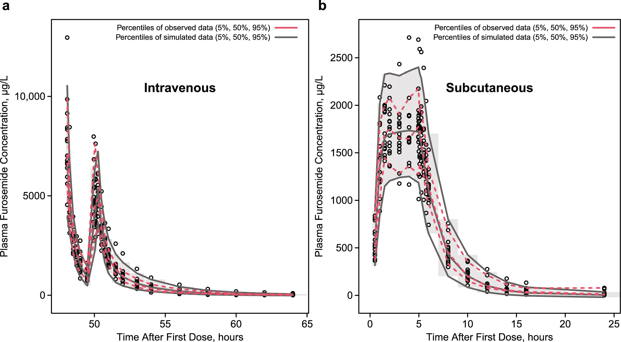
2.3 Illustration of the Novel Evaluation Approach on an Example PBPK Model

To illustrate the application of the CI of predicted-to-observed GMRs as a validation step, we validated an existing PBPK model for midazolam against published PK data from healthy adults. In the following subsections, the model specification and validation of this example PBPK model are described.

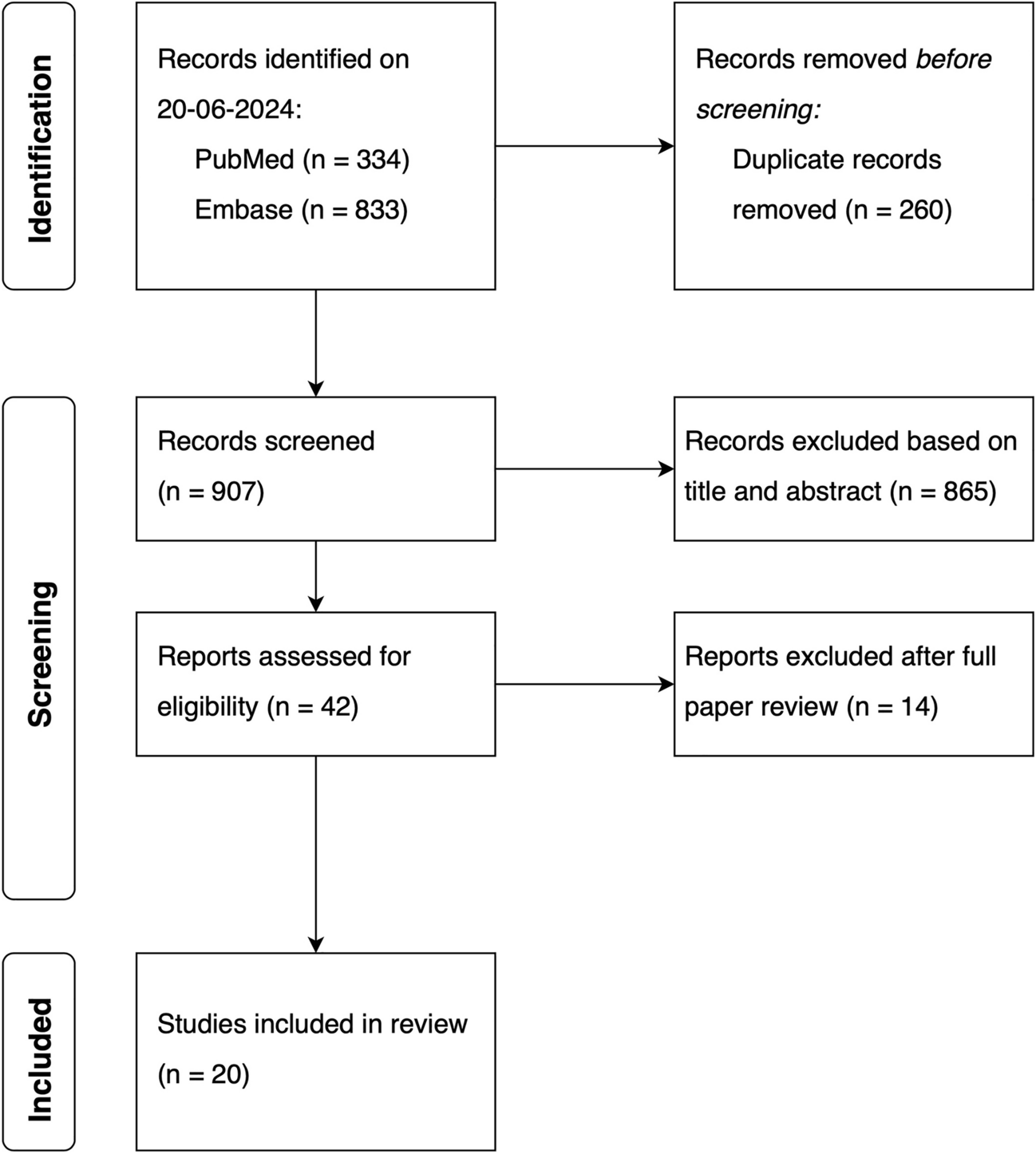
2.3.1 Midazolam Clinical PK Data

Midazolam was chosen because it has been widely investigated as its clearance is considered a probe marker to determine cytochrome P450 3A activity [21]. Additionally, a well-established PBPK model is available. A standardized search query was used to search for healthy adult PK data (detailed in the ESM). Titles and abstracts were screened for healthy volunteer midazolam PK studies. To illustrate the novel predictive performance criterion, we searched for papers with I-LD and contacted research groups to share raw PK data of published papers with aggregate PK parameters.

For I-LD sets, we only identified two older papers with individual-level PK data [22, 23]. Both papers reported a midazolam PK study with six subjects. We selected Smith et al. [22] to illustrate our novel validation approach, as this paper shared more individual characteristics compared with Heizmann et al. [23]. The characteristics of the subjects of the Smith et al. data set are given in Table S5 of the ESM. In addition, Cleary et al. [24] contributed to our study by testing our I-LD and G-LD approach on their healthy volunteer data receiving an oral single dose of midazolam 2 mg. The patient characteristics and study conditions are described previously [24].

For the illustration of the G-LD approach, we chose two recently published midazolam papers with more than 25 subjects [25, 26]. For an extra illustration of our approach in different scenarios, we created an additional hypothetical clinical data set to illustrate different scenarios of the use of our proposed validation approach, when individual-level PK data are available (ESM).

2.3.2 PBPK Model Specifics

To test the applicability of the novel predictive performance criterion, we used a default PBPK model for midazolam in healthy volunteers (model and compound file Simcyp® Version 22). Simulations were conducted to match the patient and study characteristics of the available clinical data sets. For the I-LD approach, a matched simulation of 100 subjects was conducted per individual observed subject with the custom trial option.

For the G-LD approach, a simulation was conducted matching the data sets in age, female ratio, drug dosing, and dosing route. A virtual trial of 10,000 subjects was simulated. The predictive performance was evaluated with the proposed metric of the G-LD approach.

2.3.3 Model Validation

Before modeling, the acceptance boundaries for model validations were established. The predicted-to-observed 90% CI of the AUC within the 0.8–1.25 range was considered acceptable. The Cmax of midazolam is known to be highly variable, especially for the intravenous application of midazolam [27, 28]. Therefore, a broader acceptance range of 0.67-fold to 1.5-fold was chosen as the acceptance criterion for Cmax. As motivated earlier, the same 1.5-fold was chosen as an acceptance criterion for t1/2.

For the model evaluation, simulations were conducted to match the data sets of the published papers and the hypothetical clinical study. The hypothetical clinical study was used to illustrate possible scenarios of model evaluation, when more PK IL-D are available (described in the ESM). The predictive performance of the model was validated with the published data sets following the I-LD approach and the G-LD approach. Description of PK parameters are illustrated in Tables S6 and S7 of the ESM. Pharmacokinetic parameters of the cohort of Cleary et al. are described previously [24].