Protein purification

GST-tagged RECQL51–620 was expressed in E. coli BL21-CodonPlus (DE3)-RIL cells (Stratagene) for 16 h at 18 °C and the cells were lysed with a cell disrupter (Avestin)22. The clarified lysate was loaded onto a glutathione Sepharose 4 fast-flow column equilibrated in RECQL5 buffer (20 mM Tris pH 8.0, 150 mM NaCl, 10% glycerol and 1 mM dithiothreitol (DTT)) and eluted with a linear gradient to 20 mM glutathione. The GST tag was cut with PreScission protease during dialysis for 14 h. The protein was subsequently purified using HiTrap Heparin HP and Superdex 200 columns (Cytiva) in RECQL5 buffer.

Human Pol II was purified according to a published protocol40. HeLa nuclei (114-L culture) was ground under liquid nitrogen using a mortar and pestle and then slowly resuspended in buffer A (cold 50 mM Tris-HCl pH 7.9, 5 mM MgCl2, 0.5 mM ethylenediaminetetraacetic acid (EDTA), 25% glycerol, 5 mM DTT, 1 mM sodium metabisulfite and 1 mM phenylmethylsulfonyl fluoride (PMSF), supplemented with complete EDTA-free protease inhibitor cocktail (Roche)). After sonicating the resuspension for 2 min with stirring, (NH4)2SO4 was added to a final concentration of 0.3 M. The mixture was further sonicated to reduce viscosity and then clarified by centrifugation (125,000g, 90 min, 4 °C, Ti45 rotor). The supernatant was adjusted to the conductivity of 0.1 M (NH4)2SO4 buffer through slow addition of buffer A. Then, a 42% (NH4)2SO4 cut was used to precipitate Pol II, followed by centrifugation (70,400g, 30 min, 4 °C, Ti45 rotor). The precipitate was resuspended in buffer B (cold 50 mM Tris-HCl pH 7.9, 0.1 mM EDTA, 25% glycerol, 2 mM DTT and 0.1 mM PMSF) with the concentration of (NH4)2SO4 adjusted to 0.15 M. The sample was applied to a DEAE52 column, which was washed with three column volumes of buffer B with 0.15 M (NH4)2SO4 before elution with buffer B with 0.4 M (NH4)2SO4. Protein-containing fractions were pooled and adjusted by dialysis to the conductivity of 0.2 M (NH4)2SO4 buffer, supplemented with 0.1% NP-40 substitute and immunoprecipitated overnight at 4 °C using anti-RPB1 antibody (clone 8WG16, Biolegend) crosslinked to protein G Sepharose fast-flow resin (Cytiva). The resin was washed three times with buffer C (cold 25 mM HEPES pH 7.9, 0.2 mM EDTA, 10% glycerol, 2 mM DTT, 0.1 mM PMSF and 0.05% NP-40 substitute) with 0.5 M (NH4)2SO4, followed by two washes with buffer C with 0.2 M (NH4)2SO4. Pol II was eluted through four sequential incubations with buffer C supplemented with 0.23 M (NH4)2SO4 and 1 mg ml−1 RPB1 triheptapeptide repeat (sequence: (YSPTSPS)3). Concentrated eluate was flash-frozen in liquid N2. An SDS–PAGE gel of purified proteins is shown in Extended Data Fig. 7b.

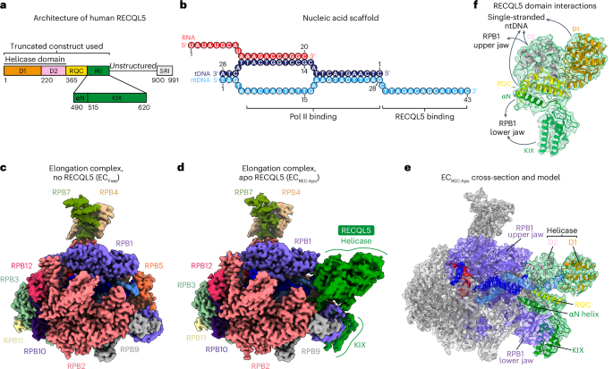
Preparation of ECREC-Apo complex

For purification of ECREC-Apo (Pol II bound to the nucleic acid scaffold and RECQL51–620-D157A with no nucleotide), Pol II was incubated first with a tenfold molar excess of the nucleic acid scaffold and then with a tenfold molar excess of RECQL5 while immobilized to the anti-RPB1–protein G resin during the Pol II purification procedure described above22. The resin was washed and the ECREC-Apo complex was eluted with RPB1 triheptapeptide repeat. Then, the complex was diluted with transcription buffer (20 mM HEPES pH 8.0, 4 mM MgCl2, 50 mM KCl, 0.05% NP-40 substitute and 1 mM Tris-(2-carboxyethyl)phosphine (TCEP)) and crosslinked with 0.02% glutaraldehyde for 10 min, followed by quenching with 100 mM Tris. Complex was then aliquoted and flash-frozen with liquid N2.

Preparation of ECREC-AMPPNP and ECREC-ADP complexes

Nucleotide-bound complexes were assembled and purified using a pulldown strategy (Extended Data Fig. 7a). First, tDNA (5′-CTCAAGTACTTACGCCTGGTCATTACTA-3′) and RNA (5′-UAUAUGCAUAAAGACCAGGC-3′) were annealed by incubating at 90 °C for 5 min and then cooling to 4 °C at a rate of 0.2 °C s−1. Pol II (diluted from 513 nM stock) was mixed with the tDNA–RNA hybrid and incubated at room temperature for 20 min. Then, desthiobiotinylated ntDNA (5′-/5deSBioTEG/TAGTAAACTAGTATTGAAAGTACTTGAGCTTAGACAGCATGTC-3′) was added and the mixture was incubated at room temperature for 20 min. All oligonucleotides were purchased from Integrated DNA Technologies. Finally, RECQL51–620 and nucleotide were added and the mixture was incubated at room temperature for 20 min. Because D157 stabilizes bound ADP through water-mediated interactions with the coordinated Mg2+ ion34, we used wild-type RECQL5 for these studies instead of the D157A mutant. The final mixture contained 350 nM Pol II, 350 nM nucleic acid scaffold, 7 μM RECQL5 and 1 mM AMPPNP or ADP, diluted in transcription buffer. After the incubation, Dynabeads MyOne Streptavidin T1 was added (6.25 μl of beads per 12.5 μl of input) and the mixture was incubated at room temperature for 75 min. The beads were washed twice with transcription buffer containing 1 mM of AMPPNP or ADP, as appropriate. Then, the complex was eluted by incubating the beads twice with elution buffer (20 mM HEPES pH 8.0, 4 mM MgCl2, 50 mM KCl, 0.05% NP-40 substitute, 1 mM TCEP, 5 mM biotin, 3% trehalose and 1 mM AMPPNP or ADP) at 37 °C for 15 min. The eluted complex was crosslinked with 0.02% glutaraldehyde at room temperature for 10 min and quenched by incubating with 100 mM Tris-HCl pH 8.0 at room temperature for 5 min. The crosslinked complexes were used to prepare cryo-EM grids on the same day.

Cryo-EM sample preparation

Cryo-EM specimens were deposited on graphene oxide (GO)-coated41 Quantifoil grids (1.2/1.3 300-mesh, carbon on gold). Grids were cleaned with chloroform, glow-discharged using a Tergeo-EM plasma cleaner (PIE Scientific), incubated for 2 min with 1 mg ml−1 polyethylenimine (Polysciences) in 25 mM HEPES pH 7.9, washed twice with H2O and air-dried. Then, grids were incubated for 2 min with 0.2 mg ml−1 GO stock solution, washed twice with H2O and air-dried. To prepare the GO stock solution, we diluted GO in 1:2 methanol and H2O (v/v), sonicated the mixture, centrifuged at 4,000g for 10 min (to remove small GO sheets), resuspended the pellet in 1:2 methanol and H2O (v/v), further sonicated the mixture and finally collected the supernatant after centrifugation at 1,000g for 1 min (to remove GO aggregates). We found that a 1:2 methanol and H2O (v/v) solution facilitated the deposition of a continuous GO layer on the grid. Grids were either used on the same day or saved and gently glow-discharged before use. Onto each grid, 3.5 μl of sample was deposited, followed by incubation for 30 s at 22 °C with 100% humidity in a Vitrobot Mark IV (Thermo Fisher Scientific). Then, the grid was blotted for 10 s with a blot force of 10 and vitrified by plunging into liquid ethane with a liquid N2 bath.

Cryo-EM data collection

All cryo-EM data were acquired as dose-fractionated videos with a 300-kV Titan Krios G3 cryo-EM instrument (Thermo Fisher Scientific) using a K3 direct electron detector (Gatan). A total exposure dose of 50 e− per Å2 fractionated across 50 frames was used during video frame recording, with defocus values ranging from approximately −0.8 to −1.8 µm. All data collection processes were automatically controlled using SerialEM42 and parameters are summarized in Table 1.

For the ECREC-Apo sample, 6,190 videos (dataset 1, EMPIAR-12711) were collected in super-resolution counting mode at ×81,000 magnification using correlated double sampling (CDS) and a super-resolution pixel size of 0.525 Å per pixel. From dataset 1, the ECREC-Apo, ECFree and ECREC-Apo (IRI-focused) structures were produced as described below.

For the ECREC-AMPPNP and ECREC-ADP complexes, data were acquired in the same instrument as described above but using non-CDS and non-super-resolution mode to increase throughput at ×81,000 magnification with a physical pixel size of 1.048 Å per pixel. For ECREC-AMPPNP and ECREC-ADP, a total of 12,100 videos (dataset 2, EMPIAR-12721) and 9,048 videos (dataset 3, EMPIAR-12722) were collected, respectively.

Cryo-EM image processing

Data processing of all images was conducted using cryoSPARC (version 4.5.3)43,44 and RELION (version 5)45,46 software, as detailed in Extended Data Figs. 1, 3, 5, 8 and 9. For simplicity, we describe in detail the data analysis workflow followed for dataset 1 (ECFree, ECREC-Apo and ECREC-Apo (IRI-focused) structures). We note that the analyses for datasets 2 and 3 (ECREC-AMPPNP and ECREC-ADP structures, respectively) were performed following similar workflows as for ECREC-Apo.

Initial dataset 1 processing

For dataset 1, the 6,190 video frames collected were aligned using patch motion correction within cryoSPARC43,44. Then, defocus estimation and contrast transfer function (CTF) fitting were performed using patch CTF estimation. In the corrected micrographs, we could readily observe particles with the size and features expected for Pol II ECs (Extended Data Fig. 2a).

A preliminary round of data processing was performed on 100 randomly selected micrographs, where particles were picked using the blob picker algorithm. Later, multiple rounds of two-dimensional (2D) classification and particle selection cycles were carried out to obtain suitable 2D templates for the following template picker job on all micrographs. Three subsequent rounds of 2D classification and particle selection cycles resulted in a set of 2,240,800 particles, from which 300,000 particles were randomly selected to perform an ab initio 3D reconstruction (n = 3). Two of three 3D ab initio maps were used as references to run a heterogeneous refinement using the full particle set (n = 4). From these classes, one particular class, containing 39.1% of the population (875,262 particles), showed defined structural features, while the other classes displayed broken complexes and/or poor low-resolution reconstructions. The particles corresponding to the best class were re-extracted using a box size of 320 pixels × 320 pixels (without binning), resulting in 871,524 particles (duplicate particles removed), and further subjected to a homogeneous refinement job, obtaining a 3D reconstruction at 2.4-Å overall resolution (Fourier shell correlation (FSC) = 0.143). At low-threshold levels, two fuzzy regions appeared next to the EC, resembling the positioning of the RECQL5 helicase (region A) and KIX domains (region B) observed in the low-resolution cryo-EM structure of this complex reported previously by our group22 (Extended Data Fig. 3). These ill-defined densities suggested a large degree of local heterogeneity or partial occupancy of RECQL5, which was quite difficult to sort out by standard classification methods. Therefore, we implemented the data analysis pipeline detailed below.

ECREC-Apo processing

The 871,524 particles in cryoSPARC were exported to RELION45,46 and subjected to 3D refinement. The RECQL5 helicase domain appeared notably less stable than the KIX domain. Therefore, we aimed first to resolve the local heterogeneity in the helicase domain (region A).

Using the volume segmentation tool in ChimeraX47,48 and the mask creation job in RELION, we generated a binary mask involving the region assigned to the RECQL5 helicase domain. We then performed a particle subtraction job to keep the signal inside the mask, while simultaneously recentering the subtracted particles on the mask and reboxing them to a box size of 180 pixels × 180 pixels. Then, using the relion_reconstruct program, we backprojected the subtracted particles to generate a low-pass-filtered 3D reconstruction to be used as a 3D reference for the next 3D classification job. This 3D classification job was performed without alignment, applying a contoured mask, generating four (n = 4) classes and using a T value of 15 and blush regularization. One of the four classes, containing 23.7% of the population (206,338 particles) and displaying better defined features, was selected and subjected to subtraction reversion to recover the full particle information. The reverted particles were then backprojected to generate a new 3D reference and then subjected to 3D refinement resulting in a reconstruction at 3.3-Å overall resolution. In this map, the RECQL5 helicase domain showed substantial improvement (interestingly, the KIX domain density also improved) and defined structural features started to become apparent. We followed up with an additional round of this strategy; however, in the second round of 3D classification without alignment, the T value was increased to 500. We suspected that a larger T value would be helpful because more relative weight would be considered on the actual experimental data (particles) along the classification cycles. One major class, accounting for 42.1% of the population (86,831 particles) and displaying clear secondary structure features, was selected and subjected to subtraction reversion, backprojection and 3D refinement (same as in the first cycle). The resulting reconstruction displayed a well-defined RECQL5, although some fuzziness was still observed for the helicase D1 subdomain (orientation in Fig. 1a). Therefore, we performed two additional rounds of this particle subtraction, 3D classification, subtraction reversion and 3D refinement cycle to improve the helicase D1 subdomain region. To this aim, different combinations of particle reboxing sizes and T values were used because of the smaller region under analysis. Ultimately, 24,323 particles were used to obtain the final cryo-EM reconstruction of ECREC-Apo at 3.2-Å overall resolution (FSC = 0.143) (Extended Data Fig. 2c). In this map, the Pol II EC core had the highest local resolution, while the fully visible RECQL5 helicase and KIX domain regions had local resolutions ranging between 3.7 Å and 5.9 Å. The final cryo-EM reconstruction was postprocessed using the DeepEMhancer sharpening program49.

The data analysis approach described above enabled us to improve the helicase domain resolution within the context of the full complex and was also used for ECREC-AMPPNP and ECREC-ADP. For the purpose of elucidating molecular interactions between RECQL5 and the Pol II EC, this workflow worked better than standard approaches such as focused classification and focused refinement only, which only resulted in an improved helicase domain map isolated from the rest of the EC. By contrast, our approach allowed us to map the full RECQL51–620 construct and describe its interactions with different regions of the Pol II EC (Fig. 2).

ECREC-Apo (IRI-focused) processing

We used a similar workflow to further improve the local resolution of the RECQL5 KIX domain region (region B) (Extended Data Fig. 5). Starting over from the 871,524 particles exported to RELION, we subjected the particles to 3D refinement and then adapted our previous data analysis approach to solve the local heterogeneity in this area. By rigid-body fitting both initial Pol II EC coordinates27 (PDB 5FLM) and a RECQL5 model predicted by AlphaFold 3 (ref. 50) into the ECREC-Apo cryo-EM map, we observed that the RECQL5 IRI module (harboring the αN helix and KIX domain) is positioned to interact with the lower jaw of the Pol II RPB1 subunit. Therefore, we generated a binary mask involving both the RPB1 lower jaw and the RECQL5 IRI module regions. We then performed a particle subtraction job to keep the signal inside the mask, recenter the subtracted particles on the mask and rebox them to a box size of 180 pixels × 180 pixels. Then, we backprojected the subtracted particles to generate its own low-pass filtered 3D reconstruction to be used as a 3D reference for the next 3D classification job. This 3D classification job was performed without alignment, applying a contoured mask, generating four (n = 4) classes and using a T value equal to 20 together with blush regularization. One of these four classes, harboring 29.0% of the population (253,055 particles), displayed better features clearly observed both in the map and in the slice view representation. This class was selected and subjected to subtraction reversion to recover the full particle information. The reverted particles were then backprojected and subjected to 3D refinement, obtaining a reconstruction at 3.2-Å overall resolution. In this 3D map, a clear improvement of the RECQL5 KIX domain region was observed. Thus, we decided to perform one additional round of this particle subtraction, 3D classification, subtraction reversion and 3D refinement cycle. Ultimately, 103,215 particles were used to obtain the final cryo-EM reconstruction of the ECREC-Apo (IRI-focused) at 2.8 Å overall resolution (FSC = 0.143) (Extended Data Fig. 2d). In this map, the region of interest involving the RECQL5 KIX domain was fully visible and displayed a local resolution range of about 3.2–4.0 Å, a major improvement compared to the ECREC-Apo structure. This final cryo-EM map was then postprocessed using the DeepEMhancer sharpening program49.

ECFree processing

As mentioned above, the 2.4-Å-resolution cryo-EM map of ECREC-Apo obtained from homogeneous refinement before RELION processing showed two fuzzy regions next to the EC corresponding to the RECQL5 helicase (region A) and KIX domains (region B) (Extended Data Fig. 3). As these ill-defined densities suggested partial occupancy of RECQL5, we performed global 3D classification without alignment in cryoSPARC (Extended Data Fig. 1). From the four 3D classes generated, one class harboring 24.3% of the total population (212,196 particles) showed no density attributable to any RECQL5 domain and was, therefore, recognized as ECFree. This class population was selected and subjected to homogeneous refinement, resulting in a 2.6-Å-resolution (FSC = 0.143) cryo-EM map. Then, an additional round of 2D classification was used to remove low-resolution particles and remaining contaminants, resulting in a set of 174,428 particles. Lastly, nonuniform refinement was used to obtain the final ECFree cryo-EM structure at 2.4-Å overall resolution (FSC = 0.143) (Extended Data Fig. 2b). This final cryo-EM map was then postprocessed using the DeepEMhancer sharpening program49.

Dataset 2 and dataset 3 processing

The image processing corresponding to datasets 2 and 3 was performed following the same approach used for dataset 1 to obtain the ECREC-Apo structure. As detailed in Extended Data Figs. 8 and 9, a total of 80,622 and 17,442 particles were used to obtain the final structures of ECREC-AMPPNP (3.2-Å overall resolution, FSC = 0.143) and ECREC-ADP (3.7-Å overall resolution, FSC = 0.143), respectively. Both maps were then postprocessed independently using the DeepEMhancer sharpening program49.

Model building, refinement and validation

For the ECFree, ECREC-Apo, ECREC-AMPPNP and ECREC-ADP structures, the initial coordinates of the EC were obtained by rigid-body fitting the atomic model of the transcribing mammalian Pol II (PDB 5FLM)27 into the corresponding postprocessed maps using ChimeraX47,48. For RECQL5, the initial coordinates were obtained from different sources. For the helicase and RQC domains, the initial model was taken from the X-ray structure of the human RECQL5 in apo form (PDB 5LB8)34, whereas, for the αN helix and KIX domain, the atomic model was predicted using AlphaFold 3 (ref. 50). These RECQL5 model regions were then semiautomatically docked and rigid-body fitted into the corresponding sharpened map.

For ECREC-Apo (IRI-focused), the transcribing mammalian Pol II (PDB 5FLM)27 model and the predicted coordinates for the RECQL5 IRI module (αN helix and KIX domain) were both rigid-body fitted into the sharpened map. For subsequent model building and refinement, we only kept the coordinates corresponding to the Pol II RPB1 lower jaw (residues 1162–1305) and the RECQL5 IRI module (harboring the αN helix and KIX domain, residues 498–620) because these were the interacting regions of interest for this structure.

For each complex, the models were then iteratively rebuilt in Coot51 and refined using the real space refinement program in PHENIX52. All validation and refinement statistics are shown in Table 1. The overall fit of the models to the maps is shown in Fig. 1e,f and Supplementary Fig. 1.

The FSCs for map versus map were obtained from the half-maps for each structure considering an applied contoured mask. The FSCs for map versus model were obtained by running a validation job in PHENIX of the corresponding final refined atomic model against the unsharpened full map. A custom Python script was used to create FSC plots.

Structural visualization and interpretation

All the structural comparisons and superpositions, as well as rotation, r.m.s.d. and distance measurements were performed in ChimeraX47,48. The difference maps shown in Extended Data Fig. 7e were generated in ChimeraX as follows. First, we created a density map from the coordinates corresponding to Pol II EC and RECQL5 only, without considering the nucleotide bound; then, this map was subtracted from the corresponding full cryo-EM map for ECREC-AMPPNP or ECREC-ADP. Overall, all main figures show the sharpened cryo-EM maps and the final refined atomic models unless otherwise specified.

RNA extension assay

RNA extension assays were conducted similarly to previous studies22,53. All oligonucleotides were purchased from Integrated DNA Technologies. First, tDNA (5′-CTCAAGTACTTACGCCTGGTCATTACTA-3′) and Cy3-labeled RNA (5′-/5Cy3/UAUAUGCAUAAAGACCAGGC-3′) were annealed, mixed with Pol II and diluted in assay buffer (20 mM HEPES pH 8.0, 4 mM MgCl2, 100 mM KCl and 1 mM TCEP) and incubated for 20 min at room temperature. ntDNA (5′-TAGTAAACTAGTATTGAAAGTACTTGAGCTTAGACAGCATGTC-3′) was added and the mixture was incubated for 20 min at room temperature, followed by addition of RECQL5 (or an equivalent volume of assay buffer) and another incubation for 20 min at room temperature. Then, nucleoside triphosphates (NTPs) were added to initiate the reaction and the mixture was incubated at 30 °C. The final reactions contained 50 nM Pol II, 200 nM nucleic acid scaffold, 2 μM RECQL5 (if added) and 800 μM each of ATP, uridine triphosphate (UTP), cytidine triphosphate (CTP) and guanosine triphosphate (GTP), all diluted in assay buffer. At appropriate time points, an aliquot of the reaction was removed and quenched with an equal volume of stop buffer (6.4 M urea, 50 mM EDTA in 1× Tris–borate–EDTA (TBE) buffer). Then, proteinase K (New England Biolabs) was added to a final concentration of 0.95 μg μl−1 and the mixture was incubated at 30 °C for 15 min. An equal volume of 2× RNA loading dye (New England Biolabs) was added and the samples were heated at 70 °C for 10 min. Samples were subjected to electrophoresis using a 15% TBE–urea gel (Bio-Rad) in 0.5× TBE (150 V, 1.5 h) and imaged on a Typhoon FLA 9500 scanner (Cytiva) detecting Cy3 fluorescence. Raw images were processed by adjusting the image levels to improve the tonal range using Adobe Photoshop 2023. All adjustments were applied to the full image.

Reporting summary

Further information on research design is available in the Nature Portfolio Reporting Summary linked to this article.