Ten sets of paired, fresh-frozen femur bones (i.e., right and left femur from the same cadaver) stripped of soft tissue were obtained. The age of the cadavers ranged from 56 to 96 years. There was one male and one female from each decade of age (i.e., age in 50 s, age in 60 s). Specimens did not have a known history of conditions that would cause an altered bone status (e.g., osteoporosis, metabolic bone disease, skeletal malignancy, prior fracture, previous surgery). The femurs were stored in freezers at − 20 °F until testing was performed, at which point the femurs were allowed to thaw to room temperature.

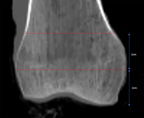
The specimens underwent standard clinical Discovery CT750 HD CT scans (General Electric, Madison, WI). Picture Archiving and Communication Systems (PACS) was used for measurements. Cortical width (the linear distance between the outer edges of the femoral cortex) and cortical index (the ratio of the sum of the medial and lateral cortical width divided by the entire width of the bone) were measured at two levels within the distal femur (Fig. 1). Measurements were performed three times by one author (JTB) and averaged. The locations (i.e., 2 and 4 cm proximal to the most distal point of the distal femoral condyles) were chosen to represent two locations of screw clusters in a standard distal femoral locking plate. HU were obtained on axial CT slices at the same two levels in the distal femur. An elliptical region of interest (ROI) was drawn as large as possible without including the cortical bone (Fig. 2).

Representative measurements of cortical width and cortical index on a mid-coronal CT image of the distal femur. Measurements are made at 2 and 4 cm proximal to the most distal aspect of the bone

Elliptical region of interests to measure CT HU drawn on axial CT slice 4 cm (A) and 2 cm (B) proximal to the end of the femur. Coronal CT (C) shows the levels of the axial slices

DXA scans were performed with Lunar iDXA (General Electric, Madison, WI, USA). Due to the absence of a specific distal femur acquisition software, scans were acquired using the orthopedic knee acquisition feature. The femurs were suspended in air using a sheet of foam insulation, to minimize contribution of mass, above a plastic container holding 6 cm of water to simulate soft tissue (Fig. 3). The approach was selected after a series of experiments using various combinations and densities of water and acrylic to mimic lean and fat respectively for a soft tissue equivalent. This method provided the best technical acquisition and image quality.

Cadaver femurs were suspended via custom radiolucent jig above 6 cm of water to simulate soft tissue during DXA acquisition

Custom regions of interest (ROIs), 2 cm in height were manually placed using index lines to measure the distance at defined locations along the distal femur (Fig. 4). The areas were again chosen to simulate the location of screw clusters. TBSortho was determined within these same ROIs using the TRIP software version 1.0.1.23.

DXA (A) and TBSortho (B) analysis of the distal femur. DXA regions of interest (ROI) were determined by manually placing a 2-cm vertical index line at the most distal tip of the femoral condyle marking the placement for the lower edge of a 2-cm horizontal region of interest. A second 2-cm ROI was stacked proximal to the initial ROI. A Subsequently, the DXA scan images were converted to DICOMs, and uploaded into TRIP software to generate TBSortho values. TBSortho ROIs were manually drawn inside the 2 DXA custom ROIs to avoid inclusion of DXA edges with the measurement. An 8-point ROI was used to outline the bone with 3 points just inside the superior and inferior DXA ROI (at each edge and in the middle), as well as a point at the center of the medial and lateral edges (B)

The femurs were rigidly fixed to a custom stabilizing jig using two 5-mm external fixator pins and a toe clamp (Fig. 5A). Five screws were placed into the bone in a configuration that simulated the use of a lateral distal femoral locking plate that is commonly used to fix distal femur fractures (4.5-mm variable angle–curved condylar plate, Depuy Synthes, Raynham, MA, USA) (Fig. 5B).

A Each cadaver femur was rigidly stabilized with transverse external fixator pins and a toe clamp. The MTS applied a constant rate of axial displacement along the axis of the bone screw, which was inserted into the lateral aspect of the distal femur, to determine screw pull-out strength. Red arrow points to screw head. B Screw configuration used for pull-out testing which simulated a lateral distal femoral locking plate. Screw 1 = anterior/distal, screw 2 = posterior/distal, screw 3 = proximal/anterior, screw 4 = proximal/posterior, screw 5 = proximal. C Anterior–posterior radiograph representing the typical position of a lateral distal femoral locking plate

The plate was placed 2 cm from the most distal surface of the lateral femoral condyle and 1 cm posterior to the anterior cortical bone, and screw positions were marked (Fig. 5B). The holes were drilled with a 4.3-mm bit and a 5.0-mm variable angle–locking screw was placed into the bone at a depth up to but not through the far cortex. A custom jig was created to hold the screw head (Fig. 5A). An axial displacement force was imposed at a constant rate of 5 mm/s (MTS Bionix system, MTS, Eden Prairie, MN, USA). The maximum force reached before failure during each trial was determined from the axial force–displacement data (MATLAB 2021b, The MathWorks, Inc., Natick, MA) (Fig. 6). Failure was defined as the peak force reached during the displacement-controlled test. The maximum pull-out force was normalized to the length of the screw within the bone.

Representative plot of the axial force and screw displacement during the displacement-controlled screw pullout tests. The peak force (*) represents the point of screw failure

Means and standard deviations, unless otherwise indicated, were used to describe the cadavers, pull-out strengths, and imaging metrics. For statistical analyses, the proximal three screw holes were averaged (proximal) and the distal two screw holes were averaged (distal). These locations within the femur correlated to the proximal and distal ROIs on the DXA. Statistical analyses were completed using the R Statistical language (version 4.3.1; R Core Team, 2023). Linear mixed effect models with the random effects for the cadaver were utilized to assess the association between imaging measures and normalized pull-out strength. The random effects model for the cadaver was included to account for the fact that both the left and right limb of a given cadaver were included in this analysis. Marginal R-squared, standardized beta, and the significance of the fixed effects from the linear mixed effect models were reported. P-value significance was set at 0.05.