Sample

The research questions were examined in a sample of 976 twins from the TwinLife Epigenetic Change Satellite (TECS) project, which is a subsample of the German twin family panel TwinLife. TwinLife is a longitudinal study of four cohorts of same-sex twin pairs and their families recruited as a representative sample from the general population of Germany [16]. The study focuses on longitudinal measures of social inequality and the potential underlying biopsychosocial mechanisms [26]. The current analysis sample consisted of 263 monozygotic (MZ) and 225 dizygotic (DZ) complete twin pairs aged 8 to 29 years at the time of the first epigenetic measurement (M = 16.0) and aged 10 to 31 years at the second measurement (M = 18.3). Zygosity was confirmed by genotyping. The age difference between cohorts was approximately 6 years. At the time of assessment, members of the four cohorts were in the ages of early adolescence, late adolescence, emerging adulthood, and young adulthood, respectively (for more details see Table 1).

Table 1 Descriptive statistics for epigenetic aging measuresDNA methylationSaliva sampling and DNA extraction

Saliva sampling for DNA extraction was conducted as a part of two TwinLife satellite projects, namely TwinSNPs and TECS. Twins and their family members were invited to participate in the molecular genetic analysis during TwinLife face-to-face interviews carried out in 2018–2020. During face-to-face interviews, interviewers offered to participate in the molecular genetic studies, which involved genotyping and epigenetic profiling. A short video explaining the study goals and procedures of the saliva sampling accompanied the recruitment procedure. The second saliva collection took place in 2021. This time, participants were contacted by mail. In addition to the invitation to participate, respondents received consent forms, saliva collection toolkits, and corresponding instructions. For all participants who provided valid consent, saliva samples were sent to the researchers at the University Hospital Bonn, Germany. The samples were collected using Oragene® saliva self-collection kits (OG-500 and OG-600; DNA Genotek, Canada) and DNA was extracted following the manufacturer’s protocol.

DNA methylation assessment

The assessment of DNA methylation profiles was conducted in a set of 2 128 samples, of which the present sample constituted a subset. The samples were randomized by age, sex, zygosity, and complete versus single twin pair across 23 plates (266 arrays) using the R package “Omixer” (version 1.4.0; [71]). The family identifier was used as a blocking variable to ensure that all samples and timepoints of a twin pair ran on the same batch/array. Bisulfite-conversion of 500 ng of DNA was performed using the D5033 EZ-96 DNA Methylation-Lightning Kit (Deep-Well; Zymo Research Corp., Irvine, USA), and methylation profiles were assessed using the Infinium MethylationEPIC BeadChip v1.0 (Illumina, San Diego, CA, USA).

Preprocessing of the methylation samples (n = 2 128) was performed following a standard pipeline by Maksimovic et al. [44] using the R package “minfi” (version 1.40.0; [3]). The following sample exclusion criteria were applied: a mean detection p value > 0.05 (n = 3) and sex mismatches between estimated sex from methylation data and confirmed phenotypic sex (n = 14). To normalize the beta values, we applied stratified quantile normalizationFootnote 4 [75], followed by BMIQ [73]. In further analysis, we removed probes containing SNPs (n = 24 038), X or Y chromosome probes (n = 16 263), cross-hybridizing probes (n = 46 867) and polymorphic probes (n = 297) according to Chen et al. [12] and McCartney et al. [47], and probes with a detection p value > 0.01 in at least one sample (n = 79 922). Afterward, beta values were transformed into M-values, and batch effects were removed using Combat [38]. For this purpose, we examined the strength of associations between three possible batches (plate, slide, and array) and the first five principal components via principal component analysis. The strongest batch effects were iteratively removed. Sample mix-ups were checked with MixupMapper [77]. The comparison of beta values with the existing genotype data (assessed using Global Screening Arrays [GSA + MD-24v3.0-Psych-24v1.1, Illumina, San Diego, CA, USA]; for further details see [14]) revealed four mix-ups. For these four cases, both samples (first and second measurements) were removed (total of n = 8 individual samples). The resulting DNA methylation dataset comprises 2 102 samples of n = 1 055 participants (among which n = 488 complete twin pairs or 976 individuals with two timepoints of DNAm data) and 698 472 probes.

The cell type composition was estimated using the R package “EpiDish” (version 2.10; [74]) and the epidish() function. Because estimated cell type proportions of saliva consisted of three (highly correlated) cell types (leukocytes, epithelial cells, and fibroblasts), we obtained the first principal component (for each epigenetic measurement, explaining 99.6% and 99.7% of cell type variation in the three estimated cell types at the first and second epigenetic measurements, respectively) to control for cell type composition in the following analyses.

Calculating epigenetic age, epigenetic age acceleration, and pace of epigenetic aging

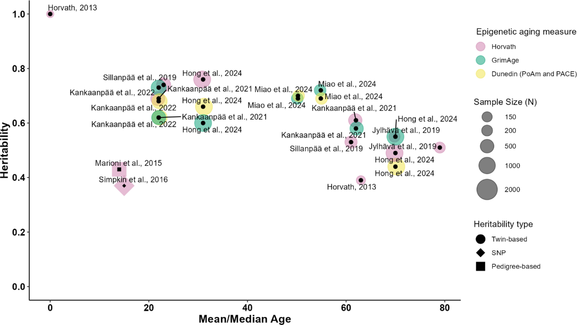
There are several types of epigenetic aging estimators, each based on a unique training model with a variable number of CpGs, source tissues, and age ranges [4, 8]. To capture potential differences in genetic and environmental contributions between different epigenetic aging measures, we selected four commonly used ones (two trained on chronological age, and two trained on biological health indicators) for our analysis: the Horvath clock [28], the PedBE clock [49], GrimAge2 (an improved version of the original GrimAge; [42, 43]), and DunedinPACE ([6]; Additional file 2: Table S2 and Figure S1). All four epigenetic aging measures have previously been shown to be associated with aging-related outcomes and to be sensitive to external drivers of aging (e.g., stress; [13, 20, 43, 48, 52, 66]). In particular, GrimAge and DunedinPACE have previously been associated with external drivers of aging in saliva of children and adolescents [18, 61, 62]. The specific background of the training sample of each epigenetic aging estimator is provided in Additional file 2: Table S2.

By the inclusion of the Horvath clock and the PedBE clock, we could address how differences in the training age range and tissue can potentially correspond to the estimates of the genetic and environmental contributions to the variance in epigenetic aging. The Horvath clock was trained as a pantissue epigenetic aging estimator in a large age range (from 0 to 101 years; [28]), while the PedBE clock was developed in buccal cells in younger age groups (from 0 to 20 years; [49]). By the inclusion of GrimAge2 and DunedinPACE, we addressed differences in the effects of the training phenotypes: both of these estimators, in contrast to Horvath and PedBE clocks, were trained on biological health indicators. In particular, GrimAge is trained on plasma proteins and smoking [43] and DunedinPACE is trained on biomarkers of organ systems integrity, such as blood pressure or serum leptin levels [6]. Finally, the inclusion of DunedinPACE allowed, in addition, to address the differences in the study design. Namely, the Horvath and PedBE clock, as well as GrimAge, are trained on the cross-sectional data, while DunedinPACE accounts for longitudinal patterns of aging.

Epigenetic aging measures were calculated based on the normalized batch-corrected beta values. The Horvath and the PedBE epigenetic age were calculated using the R package “methylclock” (version 1.01; [56]). A total of 334 (94.6%) of the original 353 Horvath clock CpG sites and all 94 CpG sites of the PedBE clock were present in the dataset. Version 2 of GrimAge was computed based on 1 029 CpG sites present in our dataset (out of 1 030 mentioned in the publication) using analysis code from Lu et al. [42] provided by A. Lu and S. Horvath via personal correspondence. The DunedinPACE values were calculated with the DunedinPACE R package (https://github.com/danbelsky/DunedinPACE/) using all of 173 CpG sites.

The four epigenetic age estimators were significantly positively correlated with chronological age (r(Horvath epigenetic age) = 0.80, p < 0.001; r(PedBE epigenetic age) = 0.77, p < 0.001; r(GrimAge) = 0.80, p < 0.001; and r(DunedinPACE) = 0.08, p < 0.001; Additional file 2: Figure S2). For the Horvath epigenetic age, the Median Absolute Error (MAE) estimates ranged from 2.75 to 3.70 (3.26–3.65 for early adolescents, from 2.75 to 2.93 for late adolescents, from 3.33 to 3.34 for emerging adults, and from 2.89 to 3.71 for young adults). For the PedBE epigenetic age, the MAE estimates ranged from 1.07 to 12.72 (2.22–2.91 for early adolescents, from 1.08 to 2.01 for late adolescents, from 6.49 to 7.51 for emerging adults, and from 11.61 to 12.72 for young adults). For GrimAge, the MAEs ranged from 19.38 to 25.60 (22.96–24.38 for early adolescents, from 25.42 to 25.60 for late adolescents, from 21.84 to 22.57 for emerging adults, and from 19.39 to 20.25 for young adults; Additional file 2: Figure S3).

Acceleration estimates for the Horvath, PedBE, and GrimAge epigenetic ages were obtained as follows: epigenetic age was regressed on chronological age (in years and decimal months), biological sex, and cell type composition within each measurement occasion. In addition, the Horvath and PedBE epigenetic ages were regressed on smoking exposure (i.e., beta values of the cg05575921 probe which has previously been shown to predict cigarette consumption in both blood and saliva [57]). This method has been chosen to overcome the missing data on smoking exposure in our sample (especially in the age group of the onset of adolescence), the limited reliability of the self-reports on smoking status and to capture, beyond active smoking, the possible effects of passive smoking exposure. The resulting residuals (i.e., Horvath Acceleration, PedBE Acceleration, and GrimAge Acceleration), defined as age acceleration (positive score) or age deceleration (negative score) according to the direction of the deviation, were used in our analyses. The DunedinPACE values were controlled for smoking probe, biological sex, and cell type composition. For DunedinPACE, a value of one reflects a pace of aging in line with one year of chronological aging. Correspondingly, values greater than one reflect an increased and values lower than one a decreased pace of aging.

Analytical strategyMain analyses

To examine the contributions of genetic and environmental factors to the variance in epigenetic aging, we applied three biometrical variance decomposition models, including (1) univariate twin models, (2) bivariate twin models across measurement occasions, and (3) univariate twin models with age as a linear continuous moderator (Additional file 3: Figure S4; [53]). MZ twins share close to 100% of their genetic makeup, while DZ twins share, on average, 50% of genetic variants that differ among humans. As a consequence, the correlation of any genetic factors is approximately 1 for MZ twins, and is assumed to approach 0.50 for additive genetic factors and 0.25 for non-additive genetic factors due to allelic dominance deviation for DZ twins. Therefore, a greater correlation within MZ twin pairs than within DZ twin pairs signals the presence of genetic influences on the variance in a specific phenotype, such as epigenetic aging in the current study.

Furthermore, both MZ and DZ twins are assumed to share some prenatal, early life familial, and extra-familial factors [9] that act to increase their resemblance beyond genetic factors. These shared environmental factors are assumed to contribute to the similarity within MZ twins to the same degree as within DZ twins. Only individually unique environmental factors are assumed to increase the dissimilarity between MZ twin siblings. Under the fulfillment of these assumptions, the classical biometrical model allows for a decomposition of the observed variance into variance attributable to genetic factors (A – additive genetic and D – non-additive genetic), environmental influences shared by twins (C), and environmental influences unique to each twin (E, including random error of measurement; [9]). For identification purposes, only three of the variance components can be estimated simultaneously in the classical twin model. Depending on the pattern of the correlations within the MZ and DZ twins, either D (if rMZ < 2 × rDZ) or C (if rMZ > 2 × rDZ) components have to be fixed to zero, resulting in the specification of either ACE or ADE models [17].

As outlined, we started our analysis with univariate twin models to decompose the variance in each epigenetic aging estimator into genetic and environmental components (Additional file 3: Figure S4a). Here, we pooled the data for the twin pairs across the two measurement occasions, resulting in a sample of 976 twin pairs for each univariate twin model. We set the variance of all variance components (A, C/D, and E) to 1 for identification purposes and ensured that the statistical conditions specified for twin modeling, namely nonsignificant differences in means and variances across co-twins and zygosity groups, were met in our sample. Then, we decided for each of the four epigenetic aging measures whether to use ACE or ADE models.

After that, among the different possible model variants (ACE, AE, CE, and E; or ADE, AE, and E), we identified the respective model that provided the best fit to the data considering model parsimony based on the Chi-square difference test. In cases where alternative models (e.g., AE and CE) were nested in one more complex model (ACE) and did not differ significantly from the latter model based on the Chi-square test, the model with a lower Akaike information criterion (AIC) was considered to fit the data better. Among the two nested models (e.g., AE vs. ADE) that differed significantly based on the Chi-square test, the model with the higher number of parameters (e.g., ADE) was considered as the model that fits the data best [22]. For the best-fitting models, we calculated the standardized coefficients with 90% confidence intervals.

In the second step, we specified bivariate twin models across the two measurement occasions (488 twin pairs) to examine the genetic and environmental sources of variance in epigenetic aging considering the repeated measurement (Additional file 3: Figure S4b). In this bivariate factor model, we analyzed the first measurement of epigenetic aging as the first variable and the second measurement of epigenetic aging as the second variable. Genetic and environmental factors were specified for each measurement occasion and were allowed to correlate over time in the sense of a correlated factors model [41]. For identification purposes, the path coefficients of the latent factors were set to 1. This model specification allowed us to estimate, along with genetic and environmental contributions to the variance in epigenetic aging at the first and second measurement occasions, the genetic and environmental covariances between the two timepoints. First, we ensured that the statistical conditions specified for twin modeling were met in our sample and specified the full model. The full model included three estimates per factor and two estimates of expected means. As was done for the univariate twin models, we have chosen among the ACE, AE, CE, and E models or, alternatively, among the ADE, AE, and E models which of these models provided the best balance between parsimony and fit. The most parsimonious model showed the lowest AIC and did not significantly fit the data worse than a more complex model based on the Chi-square difference test. Using the most parsimonious model, unstandardized and standardized variance components and genetic and environmental correlations were estimated. To examine whether or not the genetic and environmental contributions to the variance could be considered constant over time, we then restricted the genetic and environmental variance components to be equal across the first and second measurements of epigenetic aging. The model with equal variances was compared to the less constrained model with unequal variance components over time using the Chi-square difference test.

In the third step, we specified twin models with age as a linear continuous moderator of the variance components. Four age cohorts with two measures each were pooled together, resulting in eight unique age groups from 9.5 to 30 (see Table 1) with age gaps of about two and a half years between measurement occasions and age gaps of about three and a half years between the second measure of the younger cohort and the first measure of the subsequent cohort. Here, we tested whether the age of participants moderated genetic and environmental contributions to the variance in epigenetic aging to unveil possible hints on gene‒environment interactions (Additional file 3: Figure S4c; [59]). Since gene‒environment interaction effects cannot be directly assessed in classical twin models, the estimates of genetic and environmental contributions could be confounded with interaction effects [59]. In the case of interactions between additive genetic factors (A) and environmental factors that are shared by siblings reared together (C), unconsidered interaction effects would be confounded with estimates of additive genetic effects. Potential but unconsidered interaction effects between genetic factors (A) and environmental factors not shared by siblings reared together (E) would be confounded with estimates of non-shared environmental effects. While the first interaction pattern is more plausible in younger twins, who are still living in a common household, the latter is more plausible in adult years, when twins live in different households and gain more separate life experiences. As a consequence, increasing estimates of genetic contributions to the variance in epigenetic aging are more plausible in adolescence and emerging adulthood than in adulthood when accumulating effects of individually unique experiences of twins may or may not interact with genetic factors [11, 34].

To investigate the age-related moderation of the genetic and environmental variance components of epigenetic aging, age was added as a continuous linear moderator to the univariate models. This partitioned the ACE/ADE variance components into non-moderated baseline ACE/ADE components, age-moderated ACE/ADE components, a baseline intercept level, and independent linear and quadratic effects of age, producing a model with 9 parameters in total. The model was still identified as the saturated model had in total 10 measured parameters. We started with the full models (with 9 estimated parameters) and then dropped nonsignificant paths to obtain more parsimonious models with more degrees of freedom. We excluded parameters until we reached the model that fitted the data best, taking model parsimony into account (i.e., a reduced model with a lower AIC that did not fit the data significantly worse based on the Chi-square test). The variance components, confidence intervals, and standardized estimates were then derived.

Sensitivity analyses

In the final step, two sensitivity analyses were performed. As a first sensitivity analysis, we scrutinized the models of the main analysis further not controlling the epigenetic aging measures either for sex, smoking probe, or cell type composition. We repeated the univariate, bivariate, and univariate age moderation analyses, first, for all chosen epigenetic aging measures unadjusted for sex, second, for three epigenetic aging measures unadjusted for smoking, and, finally, for four epigenetic aging measures unadjusted for cell type composition. For the second sensitivity analysis, we rerun the age-moderated univariate models excluding the second timepoint to support the patterns observed in age-moderated univariate twin models using the pooled sample. By doing this, we could check if the trends in the genetic and environmental contributions to the variance in epigenetic aging across age cohorts were similar to what we observed in the main analysis with the pooled data across age cohorts and measurement occasions, ensuring that drawing the same participants twice in the analysis sample, using the first and second timepoints, did not affect the main analysis results.

The analyses were performed in R studio 2023.06.2 with R version 4.2.3. For data preparation, we used the R packages “tidyverse” [78], “ltm” [65], “dlyr” [24], and “psych” [64]. For the variance decomposition, we used “OpenMX” [54].

Power analyses

For the estimation of power to detect the model with the best balance between parsimony and fit to the data, we applied the functions proposed by Verhulst [76]. In detail, we applied the function powerValue() along with acePow() function for univariate and bivPow() for bivariate twin models. To address moderation, we applied a function developed for binary moderators, sexLimPower(), and fitted paired age groups. We formulated two possible expectations regarding genetic factors (A) based on estimates obtained in larger sample studies. Previous research suggests that the contribution of genetic factors (A) to the variance of the Horvath clock is 13% across the lifespan [39] or equals 37% at age 15 (combination with middle-aged mothers; [70]). Our expectation regarding shared environmental factors (C) was based on plots for MZ and DZ twins in Li et al. ([39]; page 8, Fig. 4, cohabitation-dependent CE model). Here, we identified approximated estimates of C for our sample’s mean age (17.1 years) of about 35%. The expectations for A and C were set to be the same across time. A power calculation for the univariate models without moderation demonstrated that 976 pairs (526 MZ and 450 DZ twin pairs) were sufficient for detecting the C component (power 0.99), while power for detecting the A component varied from 0.40 to 0.99 depending on the estimates of A. In the bivariate case without moderation, 488 pairs (263 MZ and 225 DZ twin pairs) were sufficient (0.96–0.99) to detect the C component. For the detecting of the A component, the power ranged from 0.27 to 0.99 depending on the estimates of A. Finally, power calculation for models with moderation based on the power calculation for the binary moderation demonstrated that the power to detect the A component across the age groups varied in the univariate analysis from 0.12 to 0.61. The power to detect C varied from 0.52 to 0.94.