The study was conducted and reported in adherence to the Transparent Reporting of a Multivariable Prediction Model for Individual Prognosis or Diagnosis guidelines. Our study used a publicly available EMR dataset, Medical Information Mart for Intensive Care (MIMIC-IV) [29, 30], containing postoperative ICU data from patients undergoing craniotomy. The MIMIC dataset was developed by the Laboratory for Computational Physiology at Massachusetts Institute of Technology in collaboration with Beth Israel Deaconess Medical Center and includes deidentified health care data of ICU patients [31].

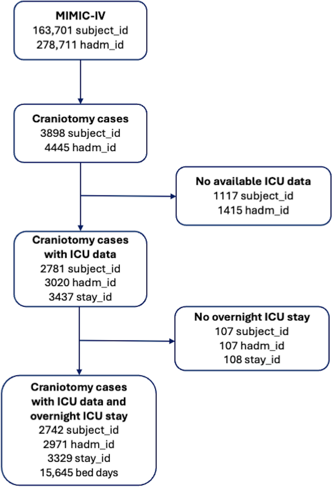
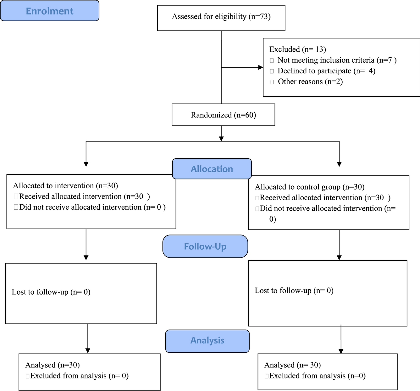
As detailed in Table 1, craniotomy cases were identified by a two-step approach using DRG and ICD procedural codes corresponding to cranial neurosurgical pathologies, such as brain tumors and aneurysms. We first screened the entire MIMIC-IV database by searching for the craniotomy and related keywords in the DRG codes. Thereafter, we extracted the list of ICD procedure codes (1,931 unique ICD codes) from all patients with at least one craniotomy-related DRG code. Finally, two neurosurgeons in our team screened these 1,931 ICD procedure codes and identified the codes that involved craniotomy (a total of 197 ICD codes). Patients with at least one of these 197 ICD codes during their hospitalization were included in our initial cohort. As detailed in Fig. 1, patients without ICU data or those who did not stay overnight in the ICU were excluded from the dataset. The final cohort was refined through a stepwise process, ensuring that the selected population consisted of patients undergoing craniotomy with at least one overnight ICU stay.

Patient selection process and inclusion–exclusion criteria flowchart. MIMIC-IV: Medical Information Mart for Intensive Care database, ICU: intensive care unit, subject_id: unique patient ID, hadm_id: unique hospital admission ID, stay_id: unique ICU stay ID

The dataset contained diverse clinical variables, including GCS scores, pupil response and size, motor strength and responsiveness, breathing patterns, comorbid disorders, and other relevant medical verbal information besides numerical data, such as laboratory results. To guarantee the quality and consistency of the data, we conducted typical preprocessing procedures, which involved addressing missing values, normalizing numerical values, and encoding categorical variables. Features with data sparsity (observed in fewer than 50 patients) were excluded to ensure reliable representation in the dataset and minimize overfitting.

The MIMIC-IV dataset includes semistructured data for clinical variables. We systematically extracted all possible variations of textual clinical descriptions and assigned numerical values. Because each variable had a finite set of possible alternatives, standardization was achieved efficiently without requiring complex neurolinguistic programming techniques. The examination results recorded as textual examination results were manually converted into numerical values through systematic grading by our clinical team. Each textual description was evaluated and assigned a clinical score on a scale reflecting best to worst outcomes, as detailed in Table 2, which comprehensively lists the clinical features used and their respective numerical scale values. The conversion process meant that the algorithm could uniformly read and analyze all clinical observations, hence improving the accuracy and reliability of the predictive ML model. Several of these scales were already in existence. Besides that, our expert neurosurgeons created others to transform verbal clinical information into numerical values, establishing a uniform measurement system for ML algorithms.

Table 3 details the laboratory results and other numerical values integrated into our ML models. The input features encompass not only these numerically encoded clinical indicators, but also additional variables related to patient demographics (e.g., age, sex) and operational parameters (e.g., time since admission, type of admission). These features provide a comprehensive dataset, enabling the model to capture many factors influencing patient outcomes.

A keyword-based screening approach was applied to radiology reports, followed by multiple refinement iterations to enhance classification accuracy. To correctly interpret negative expressions (e.g., “no midline shift”), a negation detection step was implemented to avoid misclassification. This involved recognizing phrases that explicitly indicated the absence of a condition (e.g., “no displacement of midline” or “midline within normal limits”). Table 4 outlines the positive and negative keywords used in this classification process. Positive keywords (e.g., “midline shift present,” “shift of midline structures”) were matched against report texts to identify abnormalities. In contrast, negative keywords (e.g., “no midline shift,” “midline intact”) were used to exclude false-positive results. This methodology enabled identifying radiological features with high classification accuracy (verified by manual reviews), ensuring reliable integration into the predictive model.

To ensure consistency in patient data, all clinical features used in the analysis were derived from the most relevant recorded values before discharge. Specifically, the first type of features include binary features that indicate whether an event occurred within the last 24 h (e.g., high temperature, abnormal laboratory results). The feature value is set to 1 (true) if any abnormal value was recorded within the last 24 h, regardless of the most recent measurement. If no abnormal values were recorded in this period, the feature value is set to 0 (false). The second type of features include binary features that indicate whether an event ever occurred since the admission (e.g., culture positive test result, entry of an ICD code). The feature value is set to 1 (true) if the event occurred at some point between admission and the time of prediction and 0 (false) otherwise. Finally, the third type includes continuous features indicating the latest recorded measurement (e.g., laboratory values, vital signs). Only the latest value is used if multiple values were available between admission and the prediction time. Table 5 details the timing criteria for each clinical feature, including laboratory values, GCS scores, medication administration, and oxygen delivery devices.

As demonstrated in Table 6, a comparative analysis was conducted to distinguish characteristics between the patients with and without overnight stays. This table highlights key differences in demographics, diagnoses, and procedural data, providing insights into factors influencing prolonged ICU admissions.

Because our prediction task (whether a patient will be discharged within 24 h) is a binary classification problem, we tested four different ML algorithms: logistic regression (LR), decision trees (DT), random forest (RF), and feedforward neural networks (NN). For the details of the algorithm, the reader is referred to Khaniyev et al. (2025) [32]. Of the four algorithms tested, LR and DT are considered interpretable models because they make it possible, due to their simple structure, to interpret why a specific prediction is being made based on the values of the input features. RF and NN, on the other hand, are more complex “black-box” methods that do not lend themselves to simple interpretations of the predictions. There has been, however, a growing body of literature proposing tools to “explain” the predictions of such black-box models in terms of the values of input features (e.g., Local Interpretable Model-agnostic Explanations [33], Shapley Additive Explanations [SHAP] [34], etc.). The interpretability advantage of LR and DT usually comes at the expense of model accuracy compared to black-box models such as RF and NN. In our Results section, we will briefly analyze how the tradeoff between interpretability versus accuracy plays out. The dataset was split into training (70%), validation (15%), and test (15%) samples to train, tune hyperparameters, and evaluate the models’ performance. The performance metrics used for comparison were the area under the receiver operating characteristic curve (AUC), accuracy, average precision (AP), and F1 scores. Different values for hyperparameters for each method (i.e., regularization type and strength for LR; number of layers/nodes and regularization strength for NN; maximum depth of a tree, and minimum number of samples required for each leaf for DT and RF, and number of trees/estimators for RF) were tried and the hyperparameter combination that provides the best results in the validation sample were selected for each method. During hyperparameter optimization, multiple performance metrics were evaluated, including AUC, accuracy, AP, and F1 scores.

The F1 score is a performance metric used in classification tasks, particularly in imbalanced datasets. It is the harmonic mean of precision (positive predictive value) and recall (sensitivity), ensuring a balance between false-positive and false-negative results. The F1 score ranges from 0 to 1, in which a higher value indicates better model performance by balancing precision and recall. Generally, an F1 score above 0.7 is considered strong in many practical applications, although the threshold for “strong” performance depends on the task’s complexity and class balance. A score below 0.5 typically indicates limited predictive power, especially in balanced datasets, but it may still hold value in highly imbalanced or complex prediction tasks. The F1 score is calculated using the following formula: F1 score = 2 × ([precision × recall] / [precision + recall])​. The final model selection was based on AUC, which comprehensively measures model performance across different decision thresholds.

Our model employs a sliding window approach, in which the observation window consists of all prior data up to the prediction time, and the prediction window (the subsequent 24 h from the prediction time) is for which we predict if the patient will be discharged from ICU. Each prediction is based on a patient-day unit, in which each day of ICU stay is treated as an independent observation. The sliding window approach enables continuous and dynamic risk assessment by shifting the prediction window in daily increments over time. This method allows the model to generate new predictions at regular intervals (e.g., daily), ensuring that patient data are continuously updated and assessed [35].

For simple interpretable models like LR or DT, it is relatively easy to deduce which features are contributing to the prediction made for an observation. It is not, however, as straightforward to understand how much each feature contributed to a given prediction of black-box models such as NN and RF, due to their complex nature. A large body of literature on explainable artificial intelligence [30, 33] has recently focused on alleviating the problem of explaining the predictions of black-box models. The most prominent among the explainable artificial intelligent methods is SHAP, which provides, for a given observation, how much of the predicted value is attributable to each feature. We conducted the SHAP analysis to explain the predictions of the RF model because it had the highest predictive power among the algorithms tested. SHAP values obtained for each feature of each observation are, in turn, combined to derive an overall feature importance indicating how each clinical feature influenced the RF model’s predictions for ICU discharge. Each dot represents a single observation in the SHAP summary plot. Features are color-coded to represent their values: red denotes higher feature values, whereas blue denotes lower values. The horizontal axis indicates the direction and magnitude of each feature’s impact on discharge likelihood. Features on the right with positive SHAP values increase the possibility of discharge, whereas features on the left with negative SHAP values decrease the possibility of discharge. Suppose a feature is predominantly red on the right side (e.g., “GCS – Verbal Response” [0: NO, 1: YES]); it suggests that higher values (1: YES) of this feature are favorable (i.e., higher values increase the likelihood of discharge). Conversely, if a feature is predominantly blue on the right side (e.g., O2 Delivery Device[s] [0: NO, 1: YES]), it suggests that lower values (0: NO) of this feature are favorable (i.e., lower values increase the likelihood of discharge).

We performed all statistical analyses with R (version 4.2.1) and ML training/analyses with Python (version 3.8) using the scikit-learn, tensorflow, and shap libraries. Descriptive statistics for parametric continuous variables were presented as means and standard deviations, whereas nonparametric continuous variables were summarized using medians, first and third quartiles. Categorical variables were summarized as numbers (percentages, [n ]). Group comparisons were conducted using independent t-tests for normally distributed variables and Mann–Whitney U-tests for nonnormally distributed variables. When appropriate, categorical variables were compared using χ2 or Fisher’s exact tests. A p value of less than 0.05 was considered statistically significant.