Identification of consistently dysregulated age-related genes in blood

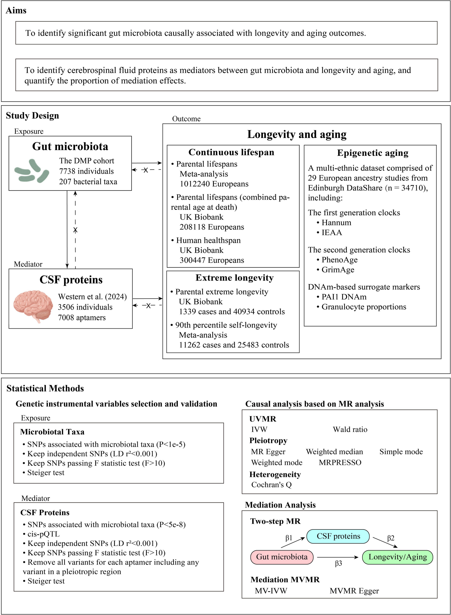
A literature search was conducted in PubMed to identify transcriptomic studies that have published lists of age-related differentially expressed genes in human blood. A cross-comparison of the lists resulted in the proposal of candidate genes for the construction of GamC (Fig. 1).

Fig. 1

Workflow for the description and characterization of GamC. The study cohorts used for GamC calculation, validation and characterization are described in the yellow boxes, indicating the number of individuals, age range, and collected material or data. CA: chronological age, ECG: electrocardiogram, GEO: Gene Expression Omnibus; GSEA: Gene Set Enrichment Analysis, y.o.: years old

Donors and samples of the study cohort

The study cohort is formed by a total of 87 Caucasian individuals from the region of Aragón (Spain) (Tables 1 and S1). The study was approved by the ethical committee for clinical research of Aragón (ID of the approval: PI17/0409 and PI18/381), and donors signed a written informed consent prior to enrollment. The study was conducted by adhering to the Declaration of Helsinki and in compliance with the European Union General Data Protection Regulation (EU 2016/679).

Table 1 Individuals in the study cohort: age range in years old (y.o.), total number of individuals, and percentage of males

Subjects self-reported their date of birth and current medical conditions and medications. They were divided into four age groups (Table 1). Young, adult, and elderly individuals were excluded from the study if they suffered from acute illness, heart disease (such as heart failure or atrial fibrillation), were taking cardiac medication, or had any other clinical condition that contraindicated exercise. However, centenarians and donors who were overweight, sedentary, or had chronic diseases such as hypertension, diabetes, or hypercholesterolemia were included in the study, since they are representative of extreme longevity or have a high prevalence in society, respectively, and thus contribute to the power of GamC. Further demographic, clinical, and biometric data are shown in Table S1.

Whole blood samples, electrocardiogram (ECG) recordings, and PA data were synchronously collected from each individual along with their CA.

Gene expression analysis by qPCR and generation of GamC

Whole blood samples were immediately processed to obtain peripheral blood mononuclear cells (PBMC) by using standard density gradient centrifugation procedures and stored at − 80 °C until use. RNA was extracted using the AllPrep DNA/RNA/miRNA Universal Kit (Quiagen). Next, 200 ng of RNA were reverse transcribed using the PrimeScript™ RT Reagent Kit (Takara). Quantitative PCR (qPCR) was performed using the NZYSupreme qPCR Green Master Mix Kit (Nzytech) with gene-specific oligonucleotide pairs (Table S2) in a Viia7 instrument (Thermo Fisher Scientific). The expression level of each age-related candidate gene was calculated as 2−ΔCt, where ΔCt = CtGene − CtReference, being CtGene the expression value of the gene and CtReference the mean expression value of two reference genes, namely, UBE2D2 and GUSB2.

The GamC of each individual was calculated as the sum of the AR and CA [29]. The AR was calculated according to previously described methods [30]. Briefly, the candidate genes with significant Pearson correlation coefficient (R) between their expression level and CA were selected to construct GamC (Fig. 1). The AR of each individual (Δi) was obtained by linear regression of the expression levels (2−ΔCt) of each gene G against CA. The regression analysis returned the residual expression level of gene G in each individual i (σG,i) and the regression factor associated with the gene G expression levels (aG). The Δi is calculated as the integration of all (N) gene-specific ΔG,i (which is in turn obtained as the ratio between σG,i and aG) (Fig. 1) (Eq. (1)):

$$_)= \frac \sum_^_= \frac \sum_^\frac_}_}$$

(1)

ECG data recording and HRV analysis

ECG recordings were obtained for all individuals in the study cohort (Fig. 1). A 12-lead high-resolution Holter ECG was acquired at rest with the 10 electrodes placed according to the manufacturer’s instructions (H12 +, Mortara Instrument, Milwaukee, WI, USA) and digitized at a sampling rate of 1000 Hz.

From the ECG recording, the heartbeats were detected and the RR interval time series were extracted using a multi-lead wavelet-based approach [31]. An operator manually verified each beat detection using a dedicated interface.

The 5-minute (min) RR interval series of each young, adult, and elderly subject was trimmed by removing 0.5 min from the beginning and the end, resulting in a final time series of 4 min. For the centenarian series, 4-min windows were defined within the 10-min recording in order to select the window with the lowest standard deviation (SD).

Linear and non-linear HRV indices were derived using algorithms developed and previously published in our research. These algorithms were implemented in MATLAB version R2021a (MATLAB, MathWorks Inc., Natick, MA, USA) [31,32,33,34]. The HRV markers extracted from the ECG are explained below:

Linear domain indices Temporal domain indices

The time series of normal RR intervals after correction for ectopic beats [32] were denoted as NN and used for subsequent analyses. Several temporal HRV indices were derived from the NN interval series including mean heart rate (MHR) calculated as the inverse of the mean NN intervals, standard deviation of NN intervals (SDNN), standard deviation of the differences between adjacent NN intervals (SDSD), root mean square of consecutive differences of adjacent NN intervals (RMSSD), and percentage of consecutive NN intervals differing by more than 50 ms (ms) divided by the total number of all NN intervals (pNN50). SDNN is considered a long-term variability measure of total HRV power, representing the variability of the ANS activity. RMSSD, SDSD, and pNN50 are short-term variability measures of parasympathetic nervous system (PNS) activity.

Frequency domain indices

From the NN interval series, the instantaneous HR signal (dHR(n)) was derived using the integral pulse frequency modulation (IPFM) model, taking into account the presence of ectopic beats [32], and sampled at 4 Hz. This signal was high pass filtered (0.03 Hz) to remove the very low frequency components (dMHR(n)) and corrected as displayed in Eq. (2) [33]. This modulating signal (\(m\)(\(n\))) carries information about the ANS activity.

$$m\left(n\right)= \frac\left(n\right)-\text(n)}(n)}$$

(2)

To estimate the spectral properties of the HRV signal, the Welch period programme was applied to m(n) using a Hamming window of 60 seconds (s) length with 30 s overlap. The power in the low frequency (LF) band, PLF, and the power in the high frequency (HF) band, PHF, were extracted by integrating the power in their respective bands: 0.04–0.15 Hz and 0.15–0.4 Hz, respectively. Normalized PLF with the total power, named as PLFn, and the ratio PLF/PHF, as an indicator of the activity of both ANS branches, were also calculated.

Non-linear indices

Non-linear HRV indices, as non-stationary measures, were also derived from the RR interval series between the individual heartbeats. Detrended fluctuation analysis (DFA) was performed by extracting the correlations between successive RR intervals at different time scales in order to measure fluctuations at different scales to detect short- and long-term correlations (α1 and α2, respectively) [35]. These markers are used to assess the complexity and adaptability of the ANS.

Finally, SD1 and SD2 were extracted from the Poincaré plot by plotting each RR interval against the previous interval to create a scatter plot. SD1 and SD2 measure the short-term and long-term beat-to-beat variability of the RR interval series, respectively. The ratio SD1/SD2 was also calculated, as the ratio between the two variabilities in the RR time series [35]. These measures are used to investigate the structure and complexity of the interbeat intervals.

Accelerometer data recording and analysis

Accelerometer data recordings were obtained for all individuals in the study cohort (Fig. 1). All individuals were asked to wear GENEActiv triaxial accelerometers (ActivInsights Ltd., Cambridgeshire, UK) for 24 h over seven consecutive days. These accelerometers were placed on the non-dominant wrist and programmed to record accelerations at 10 Hz, a frequency previously validated to classify daily activities (Zhang et al. 2012). Initialization of the GENEActiv accelerometers and retrieval of data in binary format were performed using GENEActiv PC (version 3.2) (ActivInsights Ltd., Cambridgeshire, UK).

The GGIR 3.0–2 package of the statistical programming language R v.4.3.2 [36] was used to perform accelerometer data analysis. Non-wear time detection and minimum valid time requirements for each accelerometer register were evaluated using GGIR default settings to facilitate comparability with previous studies. The minimum valid hours per day were set to sixteen, while the minimum valid days per record were set to two. Table S3 shows the relationship between the nomenclature used in this article and the variable names from the GGIR output.

Accelerometer variables were calculated [37], including the MX metrics, the average acceleration (AA), and the intensity gradient (IG). The MX metrics [38] assess the acceleration of the most active X min of a participant’s daily activity (e.g., M30 refers to the acceleration at which the most active 30 min were spent). These metrics can be used to describe the distribution of intensities over different time periods and allow for direct comparison with health-related PA guidelines. Intensity levels corresponding to the most active 1, 2, 5, 10, 15, 20, 30, 45, 60, 120, 240, 360, 480, 600, and 720 min were recorded. AA reflects the average acceleration throughout the entire measurement period and can be used as a proxy for total daily PA-related energy expenditure or PA volume [37, 39]. IG, calculated as the slope (negative) of the linear regression between the natural logarithm of time and acceleration intensity, captures the distribution of PA intensity.

Despite knowing the limitations of traditional cut-points [40, 41] due to their widespread use, the following indices were also calculated: Inactive time (IT: < 3 0 mg), time spent in light intensity PA (LPA: 30–10 0 mg), moderate intensity PA (MPA: > 100–400 mg), vigorous intensity PA (VPA: > 400 mg), and moderate-vigorous intensity PA (MVPA: > 100 mg) [42].

Exercise intervention

For the exercise intervention (Fig. 1), centenarians were randomly assigned to the control or intervention group using a computer-generated shuffle list. Participants in the control group maintained their usual PA. The intervention group performed twice per week, non-consecutive, resistance training sessions over 12 weeks (24 sessions in total). All the sessions were performed one-on-one in the gym of the geriatric nursing home and were supervised by an experienced (5 years) strength and conditioning trainer (MSc in Sports Science). After the initial assessment, participants were enrolled in a resistance exercise routine consisting of 8 different exercises according to their Functional Ambulation Classification (FAC) level [43].

Each session lasted 40–60 min, including a 10-min warm-up and 30–50 min of resistance training. The warm-up consisted of one set of eight single-joint seated exercises without resistance, 10 repetitions, and 30-s rest between exercises. Resistance training consisted of 1–3 sets of the 8 exercises routine adapted to FAC (8–10 repetitions as fast as possible, at 50–70% of the one-repetition maximum) with resting periods of 1 min between exercises and 3–5 min between sets [44]. Load, number of sets, and type of exercise routine were adjusted to the new level of physical capacity every 2 weeks.

Whole blood samples and accelerometer variables were obtained at the end of the 3-month intervention for both control and intervention groups as described above. Biochemical analysis for total cholesterol, low-density lipoproteins (LDL), triglycerides, creatine kinase (CK) and glucose levels were conducted by Centro Inmunológico de la Comunidad Valenciana (CIALAB). The accelerometer variables were obtained as described before. For each PA variable, biochemical parameter and GamC, the change in the value of each parameter after the intervention period in each individual (Pi) was calculated as the difference between after (II) and before (I) the intervention (ΔPi). Then, the median and interquartile range (IQR) of ΔPi for each PA variable, biochemical parameter and GamC were calculated for the control and intervention groups.

Validation cohorts and transcriptomic analysis

The literature search of point 2.1 and a search conducted in the GEO DataSets database, were filtered to extract studies containing readily accessible bulk tissue transcriptomic datasets from PBMC (as the study cohort) from young to elder individuals. Three independent transcriptomic datasets were obtained for analysis: cohort A (study from the USA, two age groups being 21–30 and > 70 y.o.) [45], cohort B (study from Spain, continuous ages from 19 to 93 y.o.) [46] and cohort C (study from Finland, two age groups being 19–30 and 90 y.o.) [47] (Fig. 1 and Table S4). Data were retrieved using the GEOquery package in R software, and gene annotation was applied to assign biological identifiers and filter out unannotated genes. Expression values were normalized and standardized by a quantile method for further analysis.

GamC was calculated as described above in cohorts A and B, but using the normalized and standardized expression values of the GamC-building genes. Cohort C was excluded from this calculation due to the lack of age variability in the older group.

Differential expression analysis (DEA) was performed in cohorts A and B using the Limma package in R software. Individuals were ranked by chronological age and GamC values, then divided into quartiles: young/first quartile (Q1) and elderly/fourth quartile (Q4) (Table S4). A linear model was fitted to the normalized and standardized expression data, including contrast matrices to define age-based comparisons. Log fold-change (logFC) values were estimated, and gene set enrichment analysis (GSEA) was performed using logFC values to identify enriched or depleted biological processes (GO terms) with a false discovery rate (FDR) ≤ 0.05. The top 50 GO terms with the highest absolute normalized enrichment score (NES) were manually classified into broader functional categories.

Statistical analysis

Association analysis between two variables was performed using Pearson correlation analysis for the calculation of GamC [30], its association with CA, and the association of AR with CA. Spearman correlation analysis was used for the assessment of the association between independent HRV markers and PA variables with CA or GamC and also between HRV markers with PA variables.

Comparisons between unpaired observations in two independent groups were assessed using the Mann–Whitney U test.

As normality could not be assumed in the intervention study due to the small group sizes, the Wilcoxon matched-pairs signed rank test was performed in values of control and intervention groups independently to examine differences on ΔPi of PA variables, biochemical parameters and GamC. The magnitude of the effect size (|r|) was calculated as described in Eq. (3), where Z represents the Z-score for the Wilcoxon matched-pairs signed rank test and n is the total number of observations [48].

The |r| was considered small if |r|= 0.1, medium if |r|= 0.3 and large if |r|= 0.5 [49].

All statistical analyses were performed using GraphPad Prism 8.0. The significance level was set at P ≤ 0.05 or, when adjusted for multiple-testing correction, at FDR ≤ 0.05, as conveniently indicated in the text and figure legends. The numerical value of P or FDR of every statistical test can be found in the supplementary tables.