Subjects

All procedures were approved by the Institutional Animal Care and Use Committee at Stanford University School of Medicine. C57BL/6J mice (seven males, seven females) were acquired from Jackson Laboratory. Mice were housed in a transparent cage (Innovive) in groups of five same-sex littermates before surgery, with access to an in-cage running wheel for at least 4 weeks. After surgery, mice were housed in groups of one to three same-sex littermates, with all mice per cage implanted. All mice were kept on a 12 h light–dark schedule, with experiments conducted during the light phase, and housed at ~22 °C and ~40–45% humidity. Mice were ~2.5–4.5 months of age at the time of surgery (weighing 18–31 g). Before surgery, animals had ad libitum access to food and water, and ad libitum access to food throughout the experiment. Mice were excluded from the study if they failed to perform the behavioral pre-training task described below.

Surgery for calcium indicator expression and imaging window implants

Following previously established procedures for 2P imaging of CA1 pyramidal cells6, a 3 mm diameter, ~1.3 mm long stainless steel imaging cannula (McMaster) was affixed to a circular cover glass (Warner Instruments, number 0 thickness, 3 mm diameter; Norland Optics, number 81 adhesive). During the cannula implantation procedure, animals were anesthetized through intraperitoneal injection of ketamine (~85 mg kg−1) and xylazine (~8.5 mg kg−1), maintained with inhaled 0.5–1.5% isoflurane and oxygen at a flow rate of 0.8–1 l min−1 using a standard isoflurane vaporizer. Before surgery, animals received a subcutaneous administration of ~2 mg kg−1 dexamethasone and 5–10 mg kg−1 Rimadyl (to reduce inflammation and promote analgesia, respectively). An initial hole was drilled at the viral injection site targeting the left dorsal CA1 (antero-posterior (AP), −1.94 mm; medio-lateral (ML), −1.10 to −1.30 mm), and an automated Hamilton syringe microinjector (World Precisions Instruments) with a 35-gauge needle was used to inject 500 nl adenovirus (AAV) at 50 nl min−1 in the CA1 pyramidal layer (DV, −1.33 to −1.37 mm), to express the genetically encoded calcium indicator GCaMP under the pan-neuronal synapsin promoter (AAV1-Syn-jGCaMP7f-WPRE, AddGene, viral prep 104488-AAV1, titer 2 × 1012). The needle was left in place for 10 min to allow for virus diffusion.

A 3 mm diameter circular craniotomy (center: AP, −1.95 mm; ML, −1.8 to −2.1 mm; avoiding the midline suture) was then performed over the left hippocampus using a robotic surgery drill for precision (Neurostar). During drilling, the skull was kept moist with cold sterile artificial cerebrospinal fluid. The dura was then delicately removed using a bent 30-gauge needle. To access CA1, the cortex overlying the hippocampus was aspirated with continuous irrigation of ice-cold, sterile artificial cerebrospinal fluid until the fibers of the external capsule were clearly visible and left intact. Following hemostasis, the imaging cannula was lowered into the craniotomy until the cover glass lightly contacted the external capsule. To minimize structural distortion and image tangential to the CA1 pyramidal layer, the cannula was positioned at a ~10° roll angle relative to horizontal. Cyanoacrylate adhesive was used to affix the cannula in place and cover the exposed skull surface, which was pre-scored with a number 11 scalpel before the craniotomy to provide increased surface area for adhesive binding. A headplate featuring a left-offset 7 mm diameter beveled window and lateral screw holes for attachment to the imaging rig was positioned over the imaging cannula at a matching 10° angle and cemented to the skull using Metabond dental acrylic dyed black with India ink or black acrylic powder. Following the procedure, animals were administered 1 ml of saline and 10 mg kg−1 of Baytril antibiotic, then placed on a warming blanket for recovery. A minimum 10-day recovery period was required before initiation of head-fixation and VR training.

Histology

Mice were deeply anesthetized and administered an overdose of Euthasol, then perfused transcardially with PBS followed by 4% paraformaldehyde in PBS. Brains were removed and post-fixed in paraformaldehyde for 24 h, followed by incubation in 30% sucrose in PBS for >4 days. Next, 50 µm coronal sections were cut on a cryostat, mounted on gelatin-coated slides and coverslipped with DAPI mounting medium (Vectashield). Histological images were taken on a Zeiss widefield fluorescence microscope.

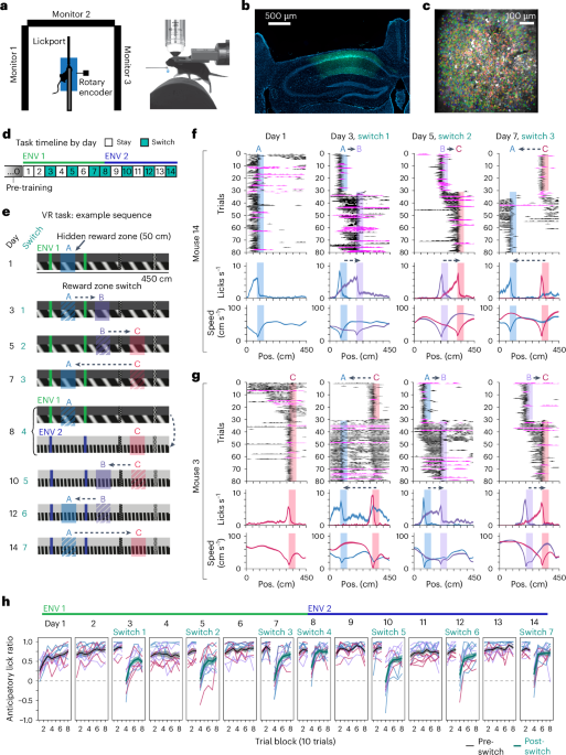
VR design

All VR tasks were designed and operated using custom code written for the Unity game engine (https://unity.com, v.2020.3.19), on a separate computer from the calcium imaging acquisition computer. Virtual environments were displayed on three 24-inch LCD monitors surrounding the mouse at 90° angles relative to each other. The VR behavior system included a rotating fixed-axis cylinder to serve as the animal’s treadmill and a rotary encoder (Yumo) to read axis rotations and record the animal’s running. A capacitive lick port, consisting of a feeding tube (Kent Scientific) wired to a capacitive sensor, detected licks and delivered sucrose water reward (5% sucrose w/v) through a gravity solenoid valve (Cole Palmer). Two separate Arduino Uno microcontrollers operated the rotary encoder and lick detection system. Behavioral data were sampled at approximately 50–75 Hz, matching the VR frame rate. Both the start of the VR task as well as each VR frame were synchronized with the ~15.5 Hz sampled imaging data by Unity-generated TTL pulses from an Arduino to the imaging computer.

Behavioral training and VR tasksHandling and pre-training

After recovery from surgery, the mice were handled for 2–3 days for 10 min each day, then acclimated to head-fixation on the cylindrical treadmill for approximately 15, 30 and 60 min over each of 3 days. To motivate behavior, mice were water-restricted to 85% or higher of their baseline body weight. Mice were weighed daily to monitor health and underwent hydration assessments (by skin tenting). Mice were acclimated to licking operantly for sucrose water rewards delivered at a minimum of 2 s intervals for 1–2 days. The water delivery system was calibrated to release ~4 μl of liquid per drop. The volume of water consumed during the experiment was measured, and supplemental water was supplied if needed up to a total of ~0.045 ml g−1 day−1 (typically 0.8–1 ml day−1, adjusted to maintain body weight), before animals were returned to their home cage each day.

Once acclimated to the lick port, mice were pre-trained on a ‘running’ task on a 350 cm virtual linear track with random black and white checkerboard walls and a white floor to collect a cued reward. The reward location was marked by two large gray towers, initially positioned 50 cm down the track. The mouse was rewarded for licking within 25 cm of the towers, otherwise, an automatic reward was given at the towers. The towers then disappeared and quickly reappeared further down the track. Covering the distance to the current reward in under 20 s increased the inter-reward distance by 10 cm, but if the mouse took longer than 30 s, the distance decreased by 10 cm, with a maximum reward location of 300 cm. Upon consistent completion of 300 cm distance in under 20 s, the automatic reward was turned off, requiring the mice to lick to receive reward. At the end of the track, the mice passed through a black curtain and into a gray ‘teleport zone’ (50 cm long) that was equiluminant with the VR environment before re-entering the track from the beginning. Once mice were reliably licking and completing 200 laps of the pre-training track within a 30–40 min period, they were advanced to the main task below and imaging (mean ± s.d., 5.8 ± 1.9 days of running pre-training across 14 mice).

Hidden reward zone task

The main ‘switch’ task involved two virtual environments similar to those previously used to study hippocampal remapping6, each with visually distinct features from the pre-training environment. Both environments consisted of a 450 cm linear track, with two colored towers (green in ENV 1, blue in ENV 2) and two patterned towers along the walls. Environments were further distinguished by the frequency of diagonal wall gratings (low, ENV 1; high, ENV 2) and color of the sky (dark gray, ENV 1; light gray, ENV 2). The reward zone was a ‘hidden’, unmarked 50 cm span at one of three possible locations along the track, each equidistantly spaced between the towers to control for proximity of each reward to visual landmarks20,32,33: zone A, 80–130 cm; zone B, 200–250 cm; zone C, 320–370 cm. Only one reward zone was ever active at a time. Reward was randomly omitted on approximately 15% of trials, determined by a random number generator for each trial. Each lap terminated in a black curtain following by a ‘teleport period’ that began with an unchanging gray display for a randomly jittered amount of time (‘jitter period’) between 1 and 5 s (5–10 s on trials following reward omissions or trials in which the mouse did not lick in the reward zone), after which the gray display began to move again for 50 cm giving the appearance of a gray ‘tunnel,’ before the mouse re-entered the virtual environment at 0 cm.

Each mouse encountered a different starting reward zone and sequence of reward zone switches, counterbalanced across mice (n = 11 mice). Most mice began the task in ENV 1 (n = 9 mice; two mice (m17 and m18) began in ENV 2). An initial reward zone (for example, A as in Fig. 1e) was acquired for days 1–2 of the task. On day 3 (switch one), the zone was moved after 30 trials to one of the two other possible locations on the track (for example, B). On the first ten trials of any new condition, including the first day and each subsequent switch, the reward was automatically delivered at the end of the zone if the mouse had not yet licked within the zone, to signal reward availability. Otherwise, the reward was delivered at the first location within the zone where the mouse licked. After these ten trials, a reward was operantly delivered for licking within the zone, and we observed that the mice often started licking before ten trials elapsed (Extended Data Fig. 1a–c). The new reward zone was maintained on day 4. On day 5 (switch two), the zone was moved to the third possible reward zone (for example, C), maintained on day 6 and moved back to the original location on day 7 (for example, A). On day 8, the reward zone switch coincided with a switch into the novel environment, where the sequence of zone switches was then reversed on the same day-to-day schedule for a total of 14 days (Fig. 1 and Extended Data Fig. 1). Each switch occurred after 30 trials.

An additional ‘fixed-condition’ cohort (n = 3 mice) experienced only ENV 1 and one fixed reward location throughout the 14 days (Extended Data Fig. 1d,f).

We targeted 80–100 trials per session with simultaneous 2P imaging (described below), with one imaging session per day (mean ± s.d., 80.5 ± 7.4 trials across 14 mice, all imaging days). The session was terminated early if the mouse ceased licking or running consistently and/or if the imaging time exceeded 50 min. Before the imaging session, mice were provided 30 ‘warm-up’ trials using the task and reward zone from the previous day to re-acclimate them to the VR setup (using the pre-training environment on day 1 of imaging). Following each daily imaging session, mice were given another ~100 training trials without imaging on the last reward zone seen in the imaging session until they acquired their daily water allotment.

2P imaging

We used a resonant-galvo scanning 2P microscope from Neurolabware with Scanbox software (https://scanbox.org, v.4.7) operated through MATLAB (Mathworks) to image the calcium activity of CA1 neurons. Excitation was achieved using 920 nm light from a tunable output femtosecond pulsed laser (Coherent Chameleon Discovery). Laser power modulation was accomplished with a Pockels cell (Conoptics). The typical excitation power, measured at the front face of the objective (Leica ×25, 1.0 NA, 2.6 mm working distance), ranged from 15–68 mW for mice m2–m7, 50–100 mW for m10 and m11, and 13–40 mW for m12–19. The task was imaged starting from day 1 for all mice except m11, for whom imaging started on day 3 owing to lower viral expression. For most animals and sessions, to minimize photodamage and photobleaching, the Pockels cell was used to reduce laser power to minimal levels between trials (during the teleport period), except for mice m11–m14 on task days 1, 7, 8 and 14, and mice m15–m19 on day 1 and all switch days, for which laser power was maintained and imaging continued throughout the teleport period. Photons were collected using Hamamatsu gated GAsP photomultiplier tubes (part H11706-401 for Neurolabware Microscopes). The imaging field of view (FOV) was collected at 1.0 magnification with unidirectional scanning at ~15.5 Hz, resulting in an approximately 0.7 × 0.7 mm FOV (512 × 796 pixels). An electrically tunable lens was used to simultaneously image deep and superficial CA1 in two mice (m17 and m18), in two planes separated by ~27 µm, with frames bidirectionally imaged at ~31 Hz interleaved in the scan for a sampling rate of ~15.5 Hz per plane. In all mice, the same FOV was acquired each session by aligning to a reference image from previous days before the start of data acquisition, with the aid of the ‘searchref’ plugin in Scanbox. This allowed us to track single cells across days.

Calcium data processing

The Suite2P software package (v.0.10.3)61 was used to perform xy motion correction (rigid and non-rigid) and identify putative cell regions of interest (ROIs). Manual curation eliminated ROIs containing multiple somata or dendrites, lacking visually obvious transients, suspected of overexpressing the calcium indicator or exhibiting high and continuous fluorescence fluctuation typical of putative interneurons. This approach yielded 155–2172 putative pyramidal neurons per session, owing to variation in imaging window implant quality and viral expression. In multi-plane imaged animals (see ‘2P imaging’), ROIs were identified separately per plane, but planes were pooled for all analyses except those in Extended Data Fig. 7. Custom code was used to follow individual ROIs across imaging sessions using the intersection over union of their pixels. The threshold for ROI matching was chosen algorithmically for each dataset such that the intersection over union for the best match for an ROI pair was always greater than the intersection over union for any second-best match.

To compute the ΔF/F (dF/F) for each ROI, baseline fluorescence was calculated within each trial independently using a maximin procedure with a 20 s sliding window. Limitation to individual trials both accounts for potential photobleaching over the session and avoids the teleport periods for sessions during which the laser power was reduced (see ‘2P imaging’). The value of dF/F was then calculated for each cell as the fluorescence minus the baseline, divided by the absolute value of the baseline, then smoothed with a two-sample (~0.129 s) s.d. Gaussian kernel. The activity rate was extracted by deconvolving dF/F with a canonical calcium kernel using the OASIS algorithm62 as used in Suite2p. We note that this deconvolution is not interpreted as a spike rate but rather as a method to eliminate the asymmetric smoothing of the calcium signal induced by indicator kinetics. Additional putative interneurons were detected for exclusion from further analysis by a Pearson correlation of >0.5 between their dF/F timeseries and the animal’s running speed, excluding 0.42 ± 0.85% of cells (mean ± s.d. across mice and days).

Statistics and reproducibility

To avoid assumptions about data distributions, we used nonparametric tests or permutation tests in most cases, except when a Shapiro–Wilk test for normality confirmed that parametric tests were reasonable. In the main text, percentages of cells classified by remapping type are reported as mean ± s.d. out of all place cells identified on the specified days. Cells were excluded from certain analyses only if they did not meet pre-established criteria as ‘place cells’ (defined in ‘Place cell identification’), to ensure that included cells provided reliable information about position in the task. Averaged data in figures are shown as mean ± s.e.m. unless otherwise indicated. For the distributions of sequence positions over days in Fig. 4 and Extended Data Fig. 4, s.e.m. shading is omitted for clarity, but the variance for these distributions is accounted for in linear mixed-effects models to quantify these plots (see ‘Linear mixed-effects models’). For data displayed as violin plots, the shape is computed as a kernel density estimate to the bounds of the data, the solid center line marks the median and additional horizontal dashed lines mark the inner quartile.

All analyses were performed in Python (v.3.8.5). Linear mixed-effects models were performed using the mixedlm method of the statsmodels package (https://www.statsmodels.org/stable/mixed_linear.html). Pairwise repeated measures t-tests were run using the pingouin package (https://pingouin-stats.org) with a Holm step-down correction for multiple comparisons. Linear regressions and Wilcoxon signed-rank and rank-sum tests were performed using the SciPy (https://scipy.org) statistics module, with linear regression confidence intervals computed with the uncertainties package (https://pypi.org/project/uncertainties). Circular statistics were performed using Astropy (https://docs.astropy.org/en/stable/stats/circ.html), pycircstat63 (https://github.com/circstat/pycircstat) and circular–circular correlation code originally written to analyze hippocampal theta phase precession64 (https://github.com/CINPLA/phase-precession). The time warp models, GLM and factorized k-means were implemented from publicly available repositories (time warp, https://github.com/ahwillia/affinewarp; GLM, https://github.com/HarveyLab/GLM_Tensorflow_2; factorized k-means, https://github.com/ahwillia/lvl).

The number of mice to include was determined by having coverage of every possible reward sequence permutation (six sequences) with at least one mouse in the switch task. In addition, our mouse sample sizes were similar to those reported in previous publications6,35. Mice were randomly selected to experience the switch task (n = 11 mice) versus the ‘fixed-condition’ task in which the reward zone was not moved (n = 3).

Estimation of anatomical location per ROI

AP and ML ROI coordinates were computed as the 2D center of mass of ROI pixels, relative to each FOV. In multi-plane imaged animals, ROIs were separated according to their deep or superficial imaging plane. To estimate deep-superficial (dorso-ventral (DV)) coordinates in single-plane animals, we acquired a z-stack scan after the day 14 task session that extended −100 µm below (−60 µm below in one mouse) to +100 µm above the FOV in the DV axis, in 2 µm steps with ~50 frames per step. Each step was independently motion-corrected as described above, and the mean of each step was used to compile the 3D z-stack array. We then took the AP projection of each ML slice of the z-stack (that is, looking at the side view of the z-stack). We minimum-filtered (4 × 0 pixel window, ML × DV) and smoothed (2 × 2 pixel s.d. Gaussian) each slice, then detected the most prominent dip in brightness in the DV axis to approximate the location of cell bodies, under the assumption that the GCaMP signal is typically absent in the nuclei and brighter in the surrounding neuropil. This yielded a per-pixel estimate of the depth of the pyramidal layer center from the dorsal surface of the z-stack, which we then smoothed (40 × 40 pixel s.d. Gaussian) to approximate the cell layer ‘curvature’ across the FOV. The curvature estimate was registered to the mean FOV of each imaging session. Given that the imaging plane transects this curvature, calculating the mean DV distance of each ROI (across pixels) from the curvature provides an estimate of where each ROI resides in the deep-to-superficial axis.

Quantification of licking behavior

The capacitive lick sensor allowed us to detect single licks. A very small number of trials with erroneous lick detection from damage to the circuit were removed from subsequent licking analysis by setting these values to NaN (~0.65% of all imaged trials, n = 81 out of 12,376 trials removed across 11 switch mice). These trials were detected by >30% of the 0.0645 s imaging frame samples in the trial containing a cumulative lick count >2, as this would have produced a sustained lick rate ≥20 Hz. Remaining lick counts were converted to a binary vector and spatially binned at the same resolution as neural activity (10 cm bins), then divided by the time occupancy in each bin to yield a lick rate. We quantified licking precision over blocks of ten trials using an anticipatory lick ratio, computed as:

$$\rm\; \rm=\frac\rm_}-\rm\rm_}}\rm_}+\rm\rm_}}$$

where Lickin is the mean lick rate in a 50 cm ‘anticipatory’ zone before the start of the reward zone and Lickout is the mean rate outside of this zone and the reward zone. The reward zone itself is thus excluded to exclude consummatory licks (Extended Data Fig. 1e). A ratio of 1 indicates perfect licking only in the anticipatory zone, a ratio of −1 indicates licking only outside of this zone and a ratio of 0 indicates chance licking everywhere, excluding the reward zone.

Place cell identification

For all neural spatial activity analyses, we excluded activity when the animal was moving at <2 cm s−1. To obtain an activity matrix of trials × position bins for each cell, we binned the 450 cm linear track into 45 bins of 10 cm each. We took the mean dF/F or deconvolved calcium activity on each trial within each position bin (note that taking the mean activity over time samples is equivalent to normalizing by the occupancy within a trial).

We defined place cells as cells with significant SI65 in either trial set 1 (pre-reward-switch) or trial set 2 (post-reward-switch) in a session. On days without a switch, we used the first and second halves of trials. For the SI, we used the deconvolved calcium activity as this reduces the asymmetry of the calcium signal. SI was calculated for calcium imaging66 as:

$$}}=\mathop\limits_^_\frac_}}_\frac_},$$

where pi is the occupancy probability in position bin i for the whole session, fi is the trial-averaged activity per position bin i and f is the mean activity over the whole session, computed as the sum of fi × pi over all N bins. To determine pi, we calculated the per-trial occupancy (number of imaging samples) in each bin divided by the total number of samples per trial, then summed the occupancy probabilities across trials and divided by the total per session. To determine the significance of the SI scores, we created a null distribution by circularly permuting the position data relative to the timeseries of each cell, by a random amount between ~1 s and the length of the trial, independently on each trial. SI was calculated from the trial-averaged activity of each shuffle, and this shuffle procedure was repeated 100 times per cell. A cell’s true SI was considered significant if it exceeded 95% of the SI scores from all shuffles within an animal, pooled across cells (more stringent than comparing to the shuffle of each individual cell67). For plotting place cell firing over trials (for example, Fig. 2), deconvolved calcium activity was normalized to the mean of each cell within a session and smoothed with a 10 cm s.d. Gaussian.

Spatial peak firing identification

To identify spatial peak firing of place cells, we used the position bin of the maximum unsmoothed, spatially binned dF/F, as this signal is the closest to the raw data, averaged across trials within a set (pre-switch or post-switch). There was no restriction to field boundaries, thus allowing cells to have multiple fields with a single identified peak.

Trial-by-trial similarity matrices

Correlation matrices were computed using the spatially binned deconvolved activity on each trial, smoothed with a 20 cm s.d. Gaussian for single cells and a 10 cm s.d. Gaussian for population vectors. This resulted in a matrix, A, of j trials × m position bins per cell. For population vectors, single-cell matrices were horizontally concatenated such that A was j trials × m position bins × n cells. Each trial was z-scored across the position axis. For single cells, the trial-by-trial correlation matrix C was computed as: \(C=\fracA^\); for population vectors: \(C=\frac-1}A^\).

Remapping category definitions

We defined the cell remapping types shown in Fig. 2 and Extended Data Fig. 2 as follows: TR, significant SI before and after the switch, with spatial peaks (see ‘Spatial peak firing identification’) ≤50 cm from each other before versus after; disappearing, significant SI before but not after the switch, with a mean spatially binned dF/F after that is less than the 50th percentile of the per-trial mean dF/F before; appearing, significant SI after but not before, with a mean spatially binned dF/F after that is greater than 1 s.d. above the mean in trials before (appearing and disappearing cells that had sufficiently reliable activity despite their rate-remapping to be captured by the RR criteria below were removed from the appearing and disappearing groups); remap near reward, significant SI before and after, with spatial peaks ≤50 cm from the starts of both reward zones; and remap far from reward, significant SI before and after, not TR, with peaks >50 cm from the start of at least one reward zone.

RR remappingQuantification of RR remapping compared to chance

For stringent statistics on putative RR remapping (Fig. 2c–i and Extended Data Fig. 2g–n), we restricted the set of included place cells to require significant SI in the pre-switch and post-switch trial sets in each session. We converted the position timeseries of the animal to periodic coordinates, setting 0 cm on the track to −π and 450 cm to π. Spatial peaks for each cell were re-computed using binned dF/F at a periodic bin size of 2π / 45 (corresponding to ~10 cm). Putative TR cells were removed by excluding cells with spatial peaks within ~0.698 radians (50 cm) of each other before versus after the switch. The periodic coordinates were then circularly rotated to align the start of each reward zone at 0, to measure the signed circular distance of spatial peaks relative to the start of each reward zone. For scatter plots of spatial peaks in Fig. 2 and Extended Data Fig. 2, points are jittered by a random amount between −π / 100 and +π / 100 for visualization only. We measured the circularly wrapped difference between relative peaks after minus before the switch, creating a distribution that can be thought of as orthogonal to the unity line in Fig. 2d,f. We compared this distribution to a ‘random-remapping’ shuffle, generated by maintaining the pre-switch peak of each cell and circularly permuting its post-switch firing 1,000 times by a random offset of 0–44 bins. To define a candidate range of RR remapping variability, we computed the circular difference between the maximum and minimum bin of the distribution of true differences between RR peaks that exceeded the upper 95% of the shuffle, divided by two and averaged across switches. In an initial cohort of n = 7 mice, this produced a mean range of ±0.656 radians (~46.9 cm) around 0, which is captured by a 50 cm threshold given our 10 cm bin size. This threshold was subsequently used to identify candidate RR remapping cells (see below).

Criteria to define RR cells

As we observed variable remapping dynamics over trials after a reward switch (Fig. 2a,b and Extended Data Fig. 2a), which could affect SI scores, we relaxed the SI criterion for RR cells such that they were required to have significant SI either before or after the switch but not necessarily both. We next implemented two criteria to identify a robust subpopulation of RR cells. First, we identified place cells with peak spatial firing relative to the reward zone start within ~0.698 radians (50 cm) of each other before versus after a reward switch (within the orange candidate zone highlighted in Fig. 2d,f), allowing for some variability in RR precision. These cells could thus include ‘remap near reward’ and ‘remap far from reward’ cells (see ‘Remapping category definitions’). Second, to reduce the influence of noise in spatial peak detection and account for the shape of the firing fields, we cross-correlated the cells’ trial-averaged, spatially binned dF/F aligned to the reward zone pre-switch versus post-switch. We predicted that RR cells should have a peak cross-correlation close to zero on this reward-centered axis. We calculated a shuffle for the cross-correlation by circularly permuting the activity in each post-switch trial by a random offset between 1 and 45 bins 500 times, requiring that the real cross-correlogram had a peak exceeding the upper 97.5% confidence interval of the shuffle and that the offset of this peak was within five bins (~50 cm) of zero. This approach provides a metric for how stable each cell’s firing is relative to reward, identifying a subpopulation of cells whose fields were maximally Pearson-correlated in periodic coordinates relative to reward, in contrast to the TR cells, which were maximally correlated relative to the original linear track coordinates (Extended Data Fig. 2o–q). Place cells that passed both criteria were defined as RR.

Relationship between distance run in the teleport zone and trial-to-trial variability

We measured the distance run in the teleport zone at the end of each trial by integrating the animal’s speed from the first frame in the teleport period to the last frame before re-entry to the start of the track. We then computed the trial-wise spatial peak error for each RR cell as the difference between the cell’s spatial peak location on each trial and its trial-averaged spatial peak location within either the trials before or after the reward switch (circular error converted back to cm). We next performed a Spearman correlation between the distance run during the teleport and the error on the following trial (Extended Data Fig. 2e,f).

Individual place field analysisPlace field definition and inclusion criteria

Using the spatially binned, deconvolved activity smoothed with a 10 cm s.d. Gaussian, excluding activity from movement speeds <2 cm s−1, candidate place fields were identified as regions of ≥20 cm that exceeded 20% of the maximum of the trial-averaged activity19 (over the 30 pre-switch trials or the final 30 post-switch trials). To include a given field, the cell was required to be significantly active within the field boundaries in at least eight (>25%) of the 30 trials, where ‘significantly active’ was defined as the raw, un-binned deconvolved activity at those positions exceeding its mean +1 s.d. across the 30 trials. For analyses of place field properties before versus after a reward switch, cells were excluded that did not have significant SI or a significant field both before and after the switch. The fraction of cell remapping types meeting these criteria on specific days is reported in Extended Data Fig. 3c. For analyses of place field width and in-field activity rate, cells were further excluded if one of their fields overlapped the first or last spatial bin of the track, as this prevented accurate detection of field boundaries that extended into the teleport zone (which was not imaged for some animals; see ‘2P imaging’). Place field width was defined as the last minus the first position bin that crossed the initial 20% activity threshold.

Coordination of remapping between fields

We assessed the alignment of the center of mass of each field to RR or TR coordinates. We first confirmed that for cells with one field before and after the switch, the field center of mass replicated the robust RR and TR remapping patterns (Extended Data Fig. 3e) observed for spatial firing peaks (Fig. 2c,d,f). Next, for the subset of cells that had exactly two fields both before and after the switch, we computed the circular–circular correlation of the offsets between fields before versus after the switch (Extended Data Fig. 3f,g).

Formation lap identification and backwards shifting

To quantify the degree of backward and forward shifting of place fields following a reward zone switch, we first identified the formation lap (trial) of each field post-switch by adapting a previously established procedure31. Within the bounds of each trial-averaged field ±10 cm after the switch, we identified trials in which the post-switch spatially binned activity exceeded its mean +1 s.d. We then found the first five-trial window with at least three trials above this threshold and took the first active trial in that window as the formation lap31. To compute the field’s center of mass on each lap with maximum spatial resolution, we used the raw deconvolved activity and position within the bounds of the trial-averaged field. We then subtracted the center of mass on the formation lap from the center of mass of the field’s mean activity in the last 30 trials of the session to quantify the degree of shift (negative values indicate a backwards shift).

Decoding of RR position

We implemented a previously developed decoder that uses circular–linear regression38 to predict the animal’s position in circular, RR coordinates from the deconvolved calcium event timeseries (at speeds of >2 cm s−1) of RR, TR or non-RR remapping neurons. The model ‘decode score’ at each timepoint t is given by \(\cos (_}-\hat}_)\), where \(_\) is the animal’s true RR position and \(\hat}_\) is the predicted RR position. A score of one indicates perfect prediction and zero indicates random prediction. We performed tenfold cross-validation in which we trained the decoder on 90% of the data and tested it on a held-out 10%, either training and testing within the trials before the switch or training on one set (before) and testing on the other set (after). Figure 3a shows decoder performance from a single cross-validation fold, considering all data from an example session. To quantify decoding accuracy compared to chance, we next downsampled the data to match occupancy at each RR position bin (bin size 2π / 45, ~10 cm), either within trials before the switch or in the last 30 trials after the switch (thereby matching trial numbers before and after). We then repeated model training and testing with 100 shuffled datasets for each session and cell subpopulation. In each shuffle, the timeseries of each cell was independently circularly shifted by a uniform random amount up to the number of samples in the session minus one. In Fig. 3b, model performance is reported as a mean decode score over time samples and cross-validation folds compared to the mean of the shuffles for each session. To evaluate decoder performance across sessions, we z-scored the decoder score of each session to its shuffle and binned the z-score as a function of RR position, then averaged across animals (Fig. 3c).

Sequence detection and quantification

For analysis of behavioral timescale sequential firing of neural subpopulations, we used the unsmoothed, spatially binned dF/F in circular track coordinates (not aligned to reward, although aligning to reward makes no difference for the circular sequence order). We sorted neurons by their peak firing positions from activity averaged over the odd trials before the switch. This sort was cross-validated6 by plotting the trial-averaged activity of the even trials before the switch (for example, left-hand columns of Fig. 4a, normalized to the mean activity of each cell within a session), then applying this sort to the trials after the switch. The sequence positions before versus after were then taken as the peak firing positions of the trial-averaged ‘even-before’ trials and the trial-averaged ‘after’ trials. Preservation of sequence order was quantified as the circular–circular correlation coefficient64 between the sequence positions before versus after. Although a P value can be directly computed for this correlation coefficient, its significance was further validated by randomly permuting the cell identities of the neurons after the switch and re-computing the correlation coefficient 1,000 times to obtain a null distribution. The observed correlation coefficient, rho, was considered significant if it was outside 95% of the null distribution using a two-tailed test. The P value was calculated as:

$$P=\frac_}_}}\right|\ge \left|}_}}\right|}+1}_}+1},$$

where \(_}_}}\right|\ge \left|}_}}\right|}\) is the number of shuffled coefficients with absolute values greater than or equal to the absolute value of the observed coefficient, and \(_}\) is the total number of shuffles. P < 0.001 indicates that the observed rho exceeded all 1,000 shuffles.

For sequences followed across days, we again used the cross-validated sort from trials before the switch (or the first half of trials if reward did not move) on the reference day (the first day in each day pair) and applied this sort to trials after the switch (or second half) on both the reference day and all trials on the target day (the second day in the pair). To measure drift between days, we computed the across-day circular–circular correlation coefficient between the sequence positions on reference day ‘after’ trials versus target day ‘before’ trials. A minimum of five followed cells in the sequence was required to compute a correlation coefficient.

To quantify the density of sequences, we divided the number of cells with peaks in each 2π / 45 position bin by the total number of place cells for that animal. These density curves were smoothed only for visualization with a one-bin s.d. Gaussian and are shown as the mean across animals per each switch day (Fig. 4 and Extended Data Figs. 4 and 5). We visualized the expected uniform distribution as the fraction of place cells in each animal’s sequence on a given switch day, divided by the number of position bins, averaged across animals.

Linear mixed-effects models

To quantify neural and behavioral changes across task experience, we used linear mixed-effects models (mixedlm method of statsmodels.formula.api) to account for variance across animals. The fixed effect was usually either the switch index or day-pair index as a continuous variable unless otherwise noted. Random effects were mouse identity. In cases of only one fixed effect term, no corrections for multiple comparisons were made. Random intercepts for each mouse were allowed; we also confirmed that including random slopes did not affect the results. When the dependent variable was reported in fractions of cells, we applied a logit transform to the fractions when a large proportion of the values were near zero. In these cases, an expit transform was applied to the model prediction to plot it with the fractional data points. In most cases, however, we chose to use the original fractions in the model for interpretability, and we confirmed that performing a logit transform on the fractions did not qualitatively change the results and only modestly changed the model fit.

Analysis of teleport periods

In the sessions for which we imaged the whole teleport period (see ‘2P imaging’), we re-identified place cells including activity during the ‘tunnel’ and part of the ‘jitter’ in the teleport period (see ‘Behavioral training and VR tasks’ for description), and re-categorized remapping types as either TR or RR from this set of place cells. Given that the length of each jitter was different, we only included spatial bins during the jitter that were occupied with fewer than ten trials missing in the session, using spatial bins of 10 cm starting at −50 cm (the start of the tunnel) up to the maximum occupied bin (range, 530–580 cm from the start of the virtual track at 0 cm). We then re-performed the population sequence analysis (see ‘Sequence detection and quantification’), up to the maximum distance occupied across mice (580 cm); note that some bins during the teleport period will include data from fewer animals (Extended Data Fig. 5). To simulate the ‘ideal’ RR remapping destination if RR fields moved by the exact amount that the reward zone moved, we added the circular difference between reward zone starts to the pre-switch peak activity position of each RR cell.

Analysis of rewarded versus omission trials

Analyses were restricted to trial sets (before or after the reward switch) that had at least three omission trials within the set.

Time warp modeling

We first fit five different time warp model types—shift, linear, piecewise one knot, piecewise two knots and piecewise three knots36—on the matrix of speed profiles within a trial set (i trials × j linear position bins × 1, expanded in the third dimension for compatibility with the time warp algorithm). These models apply warping functions of increasing nonlinear complexity to stretch and compress the data on each trial for maximal alignment36. We included both rewarded and omission trials in the fitting procedure to find the best alignment across them. Model fit was assessed using the mean squared error between the time-warped speed profile of each trial and the mean across time-warped trials (Extended Data Fig. 8a). The piecewise three knots model most often produced the best fit (lowest mean squared error) across sessions (Extended Data Fig. 8c). We therefore re-fit all sessions with piecewise three knots to ensure that model selection could not influence the results. We then applied the model transform to the deconvolved neural activity matrix for the same set of trials (i trials × j linear position bins × n neurons; excluding neural data at movement speeds of <2 cm s−1). For neural analysis in Fig. 6, we then focused on trial sets before the switch in which the reward zone was at position ‘A’ or ‘B’, because the mean rewarded versus omission speed profiles were more similar on these trials than after the switch (Extended Data Fig. 8f) or when the reward was at ‘C’ (as there is less room at the end of the track for running speed to reach its maximum from position ‘C’ on omission trials; see Extended Data Figs. 1 and 8h for examples; see Extended Data Fig. 8 for analyses of trials after the switch and for all reward zones).

Reward versus omission index

We compared neural activity on rewarded versus omission trials for RR cells with spatial peaks between the start of the reward zone and the end of the track (under the hypothesis that these cells could receive information about whether reward was received or not on that trial). Using the time warp model-transformed neural activity averaged across rewarded or omission trials within the trial set of interest, we calculated a reward versus omission index for each cell as:

$$}\; }=\frac\bar}_-\bar}_}\bar}_+\bar}_},$$

where \(\bar}_\) and \(\bar}_\) are the mean activity in position bin j averaged across rewarded trials or omission trials, respectively. Reward versus omission indices of 1 indicate an exclusive firing preference for rewarded trials, −1 indicates an exclusive preference for omission trials and 0 indicates equal firing between rewards and omissions. We confirmed that the reward versus omission index calculated from the model-transformed activity was highly correlated with the reward versus omission index calculated from the original activity (Extended Data Fig. 8e). Using a linear mixed-effects model (Extended Data Fig. 8j), we found that there was no significant change in the median reward versus omission index for each animal across days as a result of the model fit or as a result of the original mean squared error between rewarded and omission trials. We therefore combined neurons across days for presentation in Fig. 6e.

GLM

We implemented a Poisson GLM developed previously