Technology

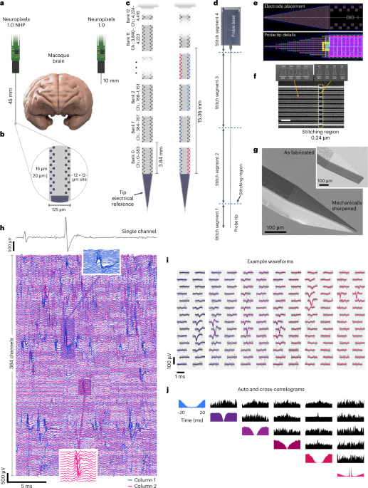
The Neuropixels 1.0 NHP probe uses the same signal-conditioning circuits as the Neuropixels 1.0 probe1, integrating 384 low-noise readout channels with programmable gain and 10-bit resolution on a 130-nm Silicon-on-Insulator CMOS platform. Within the probe shank, an array of shift-register elements and a switch matrix enable programmable selection of recording sites. The probe is fabricated as a 54-mm-long monolithic piece of silicon that integrates both the shank and the base electronics, exceeding the size of the optical reticle used to define on-chip features. We addressed this limitation by developing a method called stitching21, which precisely aligns features from different exposures between adjacent reticles.

The typical maximum size of a 130-nm CMOS chip is limited by the maximum reticle size (that is, 22 mm × 24 mm in this case) that can be exposed in a single lithography step. To build larger chips, the CMOS chip is divided into sub-blocks smaller than the reticle field, which are later used to re-compose (that is, stitch together) the complete chip by performing multiple reticle exposures per layer. The stitched boundary regions of the small design blocks are overlapped (that is, double exposed) to ensure uninterrupted metal traces from one reticle to the next, which is accounted for in the design. As multiple levels of metal wires are needed to realize and interconnect the large number of recording sites at high density, the conducting wires in the shank must be aligned between adjacent reticles for four of the six stacked aluminum metal layers. To enable stitching and to simplify photo-mask design and reuse, the probe is designed with three elements as shown in Fig. 1d: a 5-mm tip (Fig. 1e), two 20-mm middle shank segments (stitch segments 2 and 3 in Fig. 1d) and the 10-mm base segment. Four reticles are thus required to define the features on each probe. The probe base is 6 mm wide, allowing four probes to be written across these four reticles.

Four design strategies were developed to mitigate the expected degradation of signal with increased shank length: (1) the 384 metal wires connecting recording sites to the readout circuits in the base were widened relative to Neuropixels 1.0 to keep their resistance and thermal noise contribution low; (2) the spacing between the metal wires was increased to limit the signal coupling and crosstalk along the shank; (3) the power-supply wires connected to shank circuits were made wider to minimize voltage attenuation and fluctuations along the shank; and (4) the size of the decoupling capacitors was increased. The additional width and spacing of the metal lines also mitigated the impact of anticipated reticle misalignments, magnification and rotational errors in the overlap regions during stitching. Collectively, these approaches successfully enabled recording from the full 45 mm without signal degradation as a function of position (Extended Data Fig. 2).

Figure 1e shows details of the shank recording site placement and the dense CMOS layout in the shank and Fig. 1f shows a scanning electron microscope (SEM) image of the aluminium metal wires running along one of the 0.24-µm stitching regions in the shank. As a result of the double exposure of the masking photoresist at the stitching region, the wires became 24–54% narrower in this region, but remained continuous circuits without interruption.

One of the major design changes to this device, compared with the rodent probe1, was to strengthen and thicken the probe shank, which was necessary both to support the longer 45-mm shank length and to allow the probe to penetrate primate dura. To achieve this, we increased the thickness of the shank from 24 µm to 90 µm. In addition, as the increased thickness altered the bending profile of the shank, we added stress compensation layers, which help to reduce intrinsic stresses within the material in the shank and enabled us to keep bending within the same range as the rodent probes, despite the 450% increase in length.

For the data reported in the present study, we used the Neuropixels 1.0 NHP probe version with a 125 µm wide, 45 mm long shank, 4,416 selectable recording sites (pixels) and a 48 mm2 base. To facilitate insertion of the shank into the brain and to minimize dimpling and tissue damage1, the 20° top-plane, chisel-tapered shanks were mechanically ground to a 25° bevel angle on the side plane using a modified pipette microgrinder (Narishige, cat. no. EG-402). This procedure resulted in a tip sharpened along both axes (Fig. 1g). Additional discussion of insertion mechanics, methods and hardware is provided in a wiki (https://github.com/cortex-lab/neuropixels/wiki).

Scientific applications

The programmable sites of Neuropixels 1.0 NHP provide a number of advantages over existing recording technologies appropriate for primates. First, the high-channel count represents a transformative capability for large animal research. Large-scale recordings permitted rapid surveys of brain regions, enabled analyses that infer the neural state on single trials, made it practical to identify ensembles of neurons with statistically significantly correlated spike trains and reduced the number of animals and time required to perform experiments. Second, the high density of recording sites enabled high-quality, automated spike sorting22 when recording from one or both columns within a 3.84-mm bank of recording sites (Fig. 1c). The high density of sites also enabled continuous tracking of neurons in the event of drifting motion between the probe and tissue10,11, which is imperative for automated spike sorting of most real-world data22.

Third, users could choose to record with full density from one column in each of two banks, for 7.68 mm total length of high-quality, single-unit recordings, or specify alternative layouts (Extended Data Fig. 1). Programmable site selection allowed experimenters to decouple the process of optimizing a recording location from probe positioning. This capability allowed experimenters to survey neural activity along the entire probe length to map the relative positions of electrophysiological features. In addition, the programmability allowed experimenters to leave the probe in place before an experiment to improve stability during the recording.

We illustrated these collective advantages using example recordings in different macaque brain studies, including: (1) retinotopic organization of extrastriate visual cortex; (2) neural dynamics throughout the motor system; (3) face recognition in face patches of the inferotemporal (IT) cortex; and (4) neural signals underlying decision-making in the posterior parietal cortex.

Dense recordings throughout the primate visual cortex

More than half of the macaque neocortex is visual in function23 and a multitude of visual areas containing neurons with distinct feature-selective properties (for example, motion, color) lie beyond the primary visual cortex (V1). However, many of these visual areas are located deep within the convolutions of the occipital, temporal and parietal lobes (Fig. 2a). This, combined with the limitations of prior recording technologies, led to most electrophysiological studies focusing on only a subset of visual areas. Fewer than half of the identified visual areas have been well studied (for example, areas V4, MT (middle temporal)), whereas most (for example, DP (dorsal prelunate), V3A, FST (fundus of the superior temporal sulcus), PO (parieto-occipital)) have been only sparsely investigated. Given the clear similarities between the macaque and human visual systems24,25, systematic investigation across the macaque visual cortex is needed. This is practical only with technologies that enable large-scale surveys via simultaneous population recordings from both superficial and deep structures. Our initial tests with the Neuropixels 1.0 NHP probe demonstrate that it is well suited for that purpose.

Fig. 2: Single- and multi-bank recordings across multiple visual cortical areas.

a, Visual areas within macaque neocortex shown in a sagittal section. Inset, the estimated probe trajectory of one multi-bank recording. b, Spike waveforms of single neurons recorded across a single bank of (384) recording sites (3.84 mm) shown at their measured location on the probe surface. c, Population spike raster aligned to stimulus onset for units shown in b. d, Distribution of RFs of 202 visually responsive neurons across cortical depth in a single-bank recording. The arrows denote abrupt changes in RF progressions and putative visual area boundaries. e, Top view of c, illustrating the coverage of RFs across the contralateral visual field. f, The number of units identified by Kilosort 2.0 for each of the five probes recorded in the same location. Each probe was repeatedly used for up to 23 successive sessions. Units with firing rate >3 Hz are included. g, Spike waveforms of 3,029 single neurons recorded across 5 banks of recording sites (~19 mm) shown at their measured location on the probe surface. h, Heatmap of stimulus-evoked responses for all 2,729 visually responsive neurons. Each neuron is plotted at its corresponding cortical depth. The dashed black line denotes stimulus onset and the gray line at the top the 0.1-s duration. The gray shading on the right denotes depths where RFs fell on the LVM, HM or UVM. i, RF heat maps for 1,500 of the most superficial neurons, indicating visual field locations where stimuli evoked responses for each single neuron. The white crosshair in each map denotes the estimated horizontal and vertical meridians, with each map covering 26 (H) × 32 (V) d.v.a. RFs are arranged in a 42 (rows) × 36 (columns) array. Ntotal, total number of neurons; Nvisual, number of visually responsive neurons.

During individual experimental sessions, the activity of thousands of single neurons across multiple visual cortical areas could be recorded using a single NHP probe. Figure 2b,c shows the spike waveforms and rasters from one recording of 446 neurons simultaneously recorded from one bank of recording sites spanning 6–10 mm below the cortical surface. Of these neurons, 202 neurons exhibited well-defined receptive fields (RFs). As anticipated, the location of the neurons’ RFs varied as a function of the position along the probe. RFs shifted in an orderly manner for stretches of approximately 1 mm and then shifted abruptly, reflecting probable transitions between different retinotopic areas (for example, refs. 26,27,28; Fig. 2d and Extended Data Fig. 3a). Across the full depth, RFs tiled much of the contralateral hemifield and included some of the ipsilateral visual space (Fig. 2e and Extended Data Fig. 3b). When recording from up to 23 successive sessions in the same location with each probe, the number of neurons recorded varied but showed no clear decline with repeated penetrations (Fig. 2f).

In other sessions, we recorded from up to five probe banks spanning 0–19 mm beneath the pial surface (Fig. 2g) across separate blocks of trials. Using this approach, it was possible to sample from different locations without moving the probe. In one example session, 3,029 single neurons were recorded, of which 2,729 neurons were visually responsive (Fig. 2h). As with the single-bank recordings (Fig. 2d,e), neuronal RFs shifted gradually for contiguous stretches, punctuated by abrupt changes. In the example shown (Fig. 2i), RFs at more superficial sites (0–3 mm) were located at more eccentric locations of the visual field and then abruptly shifted toward the center and closer to the lower vertical meridian (LVM; ~3 mm). At the same location, neurons became more selective to the direction of motion (Extended Data Fig. 3c,d), suggesting a transition from area V4 to areas MT or MST. After that, RFs were located more centrally at the lower contralateral visual field and were observed across several millimeters. At deeper sites (~6–7 mm), smaller RFs clustered near the horizontal meridian (HM) for more than 1 mm, then quickly shifted toward the upper vertical meridian (UVM; ~8 mm). Finally, at the deepest sites (>10 mm), RFs generally became larger and much less well defined. These representations were stable throughout the duration of a session (Extended Data Fig. 3e). These data illustrate how the Neuropixels 1.0 NHP’s dense sampling and single-unit resolution facilitate large-scale and unbiased mapping of the response properties of neurons across multiple visual areas.

Stable, large-scale recording during motor behaviors

Next, we demonstrated the utility of this technology for studying multiple brain areas involved in movement control. Primary motor cortex (M1) is situated at the rostral bank of the central sulcus and extends along the precentral gyrus. Sulcal M1 contains the densest projections of descending corticomotoneuronal cells and corticospinal neurons, which collectively are understood to convey the dominant efferent signals from the brain to the periphery in primates29,30. Constraints of existing technology have led to two broad limitations in studies of the motor system.

First, motor electrophysiologists have been forced to choose between simultaneous recording from populations of superficial neurons in gyral motor cortex (PMd and rostral M1) using Utah arrays31 and, alternatively, recording fewer neurons in sulcal M1 using single-wire electrodes or passive arrays of 16–32 contacts (for example, Plexon S-probes or Microprobes Floating Microwire Arrays17). Recording from large populations of neurons in sulcal M1 has not been feasible.

Second, the motor cortex is only one part of an extensive network of cortical and subcortical structures involved in generating movement29,32. Many investigations of the motor system focus on M1 and comparatively fewer experiments have investigated neural responses from the numerous additional structures involved in planning and controlling movements, the result in part of the challenge of obtaining large-scale datasets in subcortical structures in primates. Areas such as the supplementary motor area (SMA) and the basal ganglia (BG) are understood to be important for planning and controlling movements, but investigation of the functional roles and interactions between these regions is hampered by the challenge of simultaneously recording from multiple areas.

We developed a system capable of simultaneous recordings from multiple Neuropixels 1.0 NHP probes in superficial and deep structures of rhesus macaques. We tested this approach using a task in which a monkey generated isometric forces to track the height of a scrolling path of dots (Fig. 3a; task described in ref. 33). We recorded from the primary motor and premotor cortex (M1 and PMd; Fig. 3b) while the monkey tracked a variety of force profiles (one profile per condition). Each condition was repeated across multiple trials (Fig. 3c). Single neurons exhibited a diversity of temporal patterns throughout the motor behavior (Fig. 3d–f). When ordered using Rastermap34, neurons illustrated a diversity of phase relationships with respect to the behavior (Fig. 3f). Predictions of endpoint force from neural activity (via linear regression) improved steadily as more neurons were included in the analysis and the performance did not saturate even when including all recorded neurons (360) for an example session (Fig. 3g). Thus, despite the apparent simplicity of a one-dimensional force-tracking task, neural responses are sufficiently diverse that it is necessary to sample from many hundreds of neurons to capture a complete portrait of population-level activity.

Fig. 3: Recording from the rhesus motor system.

a, Pacman isometric force-tracking task. b, Recording targets in motor cortex (left) and schematic of recording target in sulcal M1, sagittal section (right). c, Trial-averaged arm force during pacman task. d, Trial-averaged firing rate for example neurons. e, Single-trial spike raster for four example neurons. f, Trial-averaged, normalized responses of all 360 neurons for the same session as data in c–e, ordered using Rastermap34. g, Linear model force prediction accuracy as a function of the number of neurons included in the analysis. h, Spike waveforms on ten channels of four example neurons, averaged across nonoverlapping time bins that represent one-fifth of the recording duration. i, Probe drift estimating output by Kilosort 2.5 over the duration of a single motor behavioral session. Each line represents the estimate for a subset of channels.

The relative motion of the probe within the brain tissue is a major concern for the stability of neural recordings. Motor tasks represent a challenging set of conditions because movement of the body can place stresses on the implant and move the probe within the brain. With careful preparation, on most sessions we did not observe rapid probe motion due to pulse, respiration or mechanical forces from the motor task. Typically, we observed stable waveforms (Fig. 3h) and ~2–15 µm of slow drift over the course of a recording session (Fig. 3i and Extended Data Figs. 4a and 5). In some isolated cases, when the primate generated a large unexpected movement, we did observe a fast translation of the probe (for example, Extended Data Fig. 4b). However, in practice, we found that low-drift recordings could be obtained across a variety of experimental preparations in disparate brain regions (Fig. 4a–d and Extended Data Figs. 4 and 5).

Fig. 4: Example drift maps from four brain regions.

a, Top, drift map visualization of position versus time for one representative recording from the motor cortex. The darker spots indicate larger amplitude spikes. Bottom, estimate of drift calculated using Kilosort for the same recording shown above. b–d, Same visualization as shown in a for visual cortex (b), area AF (c) and area LIP (d), respectively.

Programmable site selection in the Neuropixels 1.0 NHP enables simultaneous recording from superficial and deep structures using a single probe. To illustrate this capability, we recorded from superficial motor cortex and internal globus pallidus (GPi) in the BG using 192 channels in each target location (Fig. 5a,b). Alternatively, the small form factor of the Neuropixels 1.0 NHP probes and headstages allows for dense packing of multiple probes by inserting probes along nonparallel trajectories to record from a large number of neurons in a single area. Figure 5c,d illustrates recordings from three probes in gyral PMd, yielding 673 neurons. This approach was tested on two sessions, in which we recorded from 6 and 7 probes, yielding 1,012 and 783 neurons, respectively. These yields were lower than average as a result of imperfect recording conditions unrelated to the insertion hardware. Sampling with multiple probes is also well suited for simultaneous recording from different brain areas. Figure 5e illustrates a system designed to record from M1, the GPi of the BG and the SMA, using multiple probes inserted into a single recording chamber, with representative neural responses illustrated in Fig. 5f.

Fig. 5: Simultaneous targeting of multiple brain areas with one or more probes.

a, Multi-area recording using a single probe in the motor cortex and BG (GPi), allocating 192 channels to each region via programmable site selection. b, Example raw waveforms and site selection for the recording described in a. c, Recording from many neurons within a single small target region using multiple probes inserted along convergent trajectories. d, Example waveforms of neurons recorded on probes using the apparatus shown in c. e, Recording from disparate brain regions (SMA, M1 and GPI) using three probes, all inserted along parallel trajectories. f, Example neurons recorded using the apparatus shown in e.

Face recognition in the IT cortex

Next, we demonstrated the use of the probes in the inferotemporal (IT) cortex, a brain region in the temporal lobe that is challenging to access because of its depth. The IT cortex is a critical brain region supporting high-level object recognition and has been shown to harbor several discrete networks35, each specialized for a specific class of objects. The network that was discovered first and has been most well studied in nonhuman primates is the face-patch system. This system consists of six discrete patches in each hemisphere36, which are anatomically and functionally connected. Each patch contains a large concentration of cells that respond more strongly to images of faces than to images of other objects. Studying the face-patch system has yielded many insights that have transferred to other networks in the IT cortex, including increasing view invariance going from posterior to anterior patches and a simple, linear encoding scheme35. As such, this system represents an approachable model for studying high-level object recognition37. The code for facial identity in these patches is understood well enough that images of presented faces can be accurately reconstructed from neural activity of just a few hundred neurons38.

A major remaining puzzle is how different nodes of the face-patch hierarchy interact to generate object percepts. To answer this question, it is imperative to record from large populations of neurons in multiple face patches simultaneously to observe the varying dynamics of face-patch interactions on a single-trial basis. This is essential because the same image can often invoke different object percepts on different trials39. In the present study, we recorded with one probe in each of two face patches, middle lateral (ML) and anterior fundus (AF), simultaneously (Fig. 6a). The Neuropixels 1.0 NHP probes recorded responses of 1,127 units (622 single units, 505 multi-units) across both face patches during a single session (Fig. 6a, right). A continuous segment of approximately 220 channels (2.2 mm) in ML and 190 channels (1.9 mm) in AF contained face-selective units, indicating that these extents of the probes were in the IT cortex. In ML 261 units and in AF 297 units were face selective (two-sided, two-sample Student’s t-test, threshold P < 0.05).

Fig. 6: Deep, simultaneous recordings from two face patches in the IT cortex.

a, Simultaneous targeting of two face patches. Coronal slices from MRI show inserted tungsten electrodes used to verify targeting accuracy for subsequent recordings using Neuropixels 1.0 NHP (top, face-patch ML; bottom, face-patch AF). Yellow overlays illustrate functional MRI contrast in response to faces versus objects. b, Response rasters for a single stimulus presentation of simultaneously recorded neurons in ML and AF to a monkey face, presented at t = 0. Each line in the raster corresponds to a spike from a single neuron or multi-unit cluster, including both well-isolated single units and multi-unit clusters. c, Neuropixels 1.0 NHP enabling recordings from many face cells simultaneously. These plots show the average responses (baseline subtracted and normalized) of visually responsive cells (rows) to 96 stimuli (columns) from 6 categories, including faces and other objects. Bottom, exemplar stimuli from each category. The plots included 438 cells or multi-unit clusters in ML (left) and 689 in AF (right), out of which a large proportion responded selectively to faces. Units were sorted by channel, revealing that face cells are spatially clustered across the probe. d, Coronal slice of MRI of Neuropixels probe targeting the deepest IT face-patch AM. The thick shadow is a cannula that was inserted through the dura into the brain. The thin shadow corresponds to the Neuropixels trajectory. e, Same as c, for face-patch AM, recorded in a different session.

Changing the visual stimulus to a monkey face yielded a clear visual response across both face-patch populations. We measured responses of visually responsive cells to 96 different stimuli containing faces and nonface objects (Fig. 6b,c). A majority of cells in the two patches showed clear face selectivity. Using single-wire tungsten electrodes, this dataset would have taken about 2 years to collect, but is now possible in a single 2-h experimental session38. In addition, to the gain in efficiency created by this technology, simultaneous recordings of multiple cells and multiple areas allowed for investigation of how populations encode object identity in cases of uncertain or ambiguous stimuli, where the interpretation of the stimulus may vary from trial to trial but is nevertheless highly coherent on each trial. The anatomical depth of face patches puts them far out of reach for shorter high-density probes. For example, face-patch AM (anteromedial) sits about 42 mm from the craniotomy (Fig. 6d) along a conventional insertion trajectory, but face patches in this region are still accessible using the Neuropixels 1.0 NHP probe and exhibit face-selective responses within the boundaries of AM (Fig. 6e).

Single-trial correlates of decision-making in LIP

For many cognitive functions, the processes that give rise to behavior vary across repetitions of a task. As such, technologies that enable the analysis of neural activity at single-trial resolution will be especially critical for research on cognition. Achieving this resolution is challenging because it requires recordings from many neurons that share similar functional properties.

This challenge is exemplified in perceptual decision-making, in which decisions are thought to arise through the accumulation of noisy evidence to a stopping criterion, such that their evolution is unique on each trial in a dynamic motion discrimination task (Fig. 7a; for task see ref. 40). This process is widely observed and known as drift diffusion41,42. Neural correlates of drift diffusion have been inferred from activity in the lateral intraparietal area (LIP) averaged over many decisions. LIP neurons display spatial RFs and represent the accumulated evidence for directing the gaze toward the RF. Analysis of LIP activity during single decisions has proven particularly difficult because RFs have little to no anatomical organization (Fig. 7c, top), preventing simultaneous recordings from many neurons with the same receptive field.

Fig. 7: Single-trial dynamics of a decision process in multiple brain regions.

a, Task. The monkey must decide the net direction of dynamic RDM and indicate its decision by making a saccadic eye movement, whenever ready, from the central fixation point (red) to a left-choice or right-choice target (black). The choice and response times are explained by the accumulation of noisy evidence to criterion level54. b, Simultaneous recordings in LIP and SC. Populations of neurons were recorded in LIP with a Neuropixels 1.0 NHP probe and in SC (deeper layers) with a multi-channel V-probe (Plexon). c, RFs are identified, post-hoc, from control blocks in which the monkey performed an oculomotor delayed response task55. A small fraction of the LIP neurons (top) has RFs that overlap the left-choice target (outlined in black). The SC (bottom) has a topographic map, so many neurons have overlapping RFs. The large sample size in LIP facilitates identification of neurons that respond to the same choice target in LIP and SC. d, Single-trial activity in LIP (top, n = 17) and SC (bottom, n = 15). Each trace depicts the smoothed firing rate average (Gaussian kernel, σ = 25 ms) of the 17 neurons that overlap the left-choice target (Tin) on a single trial, aligned to the onset of the motion stimulus. Rates are offset by the mean firing rate of 0.18–0.2 s after motion onset to force traces to begin at 0. The line color indicates the decision for the left-choice target or the right-choice target (Tout) on that trial. A few representative traces are highlighted for clarity. e, The same trials as in d aligned to saccade initiation, without baseline offset. Single-trial firing rates approximate drift diffusion in LIP—the accumulation of noisy evidence—whereas single-trial firing rates in SC exhibit a large saccadic burst at the time of the saccade, preceded by occasional nonsaccadic bursts.

Neuropixels recording in the LIP overcomes this challenge. These recordings yield 50–250 simultaneously recorded neurons, of which 10–35 share an RF that overlaps one of the contralateral choice targets used by the monkey to report its decision. The average activity of these target-in-RF (Tin) neurons during a single decision tracks the monkey’s accumulated evidence as it contemplates its options. The signal explains much of the variability in the monkey’s choices and reaction times43 and conforms to drift-diffusion dynamics (Fig. 7d,e, top).

Neuropixels technology also enables multi-area recordings from ensembles of neurons that share common features (Fig. 7b). For example, neurons in the deeper layers of the superior colliculus (SC) receive input from LIP and, like LIP neurons, also have spatial RFs and decision-related activity (Fig. 7c, bottom). An ideal experiment to understand how the two areas interact is to record simultaneously from populations of neurons in LIP and SC that share the same RF. This experiment is almost impossible with previous recording technology because of the lack of anatomical organization in the LIP.

This second challenge is also overcome by Neuropixels recording in the LIP, allowing for post-hoc identification of neurons in the LIP and SC with overlapping RFs (Fig. 7c). In the experiment depicted in Fig. 5, the response fields of 17 of the 203 LIP neurons overlapped the left-choice target as well as 15 simultaneously recorded neurons in the SC. Unlike LIP, single-trial analysis of the SC population revealed dynamics that are not consistent with drift diffusion (Fig. 7d,e, bottom). Instead, the SC exhibits bursting dynamics, which were found to be related to the implementation of a threshold computation44. The distinct dynamics in the LIP and SC during decision-making were observable only through single-trial analyses, the resolution of which is greatly improved with the high yield of the Neuropixels 1.0 NHP recording.

Measuring spike–spike correlation with high-density probes

Understanding how the anatomical structure of specific neural circuits implements neural computations remains an important but elusive goal of systems neuroscience. One step toward connecting disparate levels of experimental inquiry is mapping correlative measures of relative spike timing between pairs of neurons, which is indicative of either synaptic connection between two neurons or shared input drive6,13,45. This is often impractical or extremely challenging when recording from only a small number of neurons, because the likelihood of recording from a pair of neurons with a statistically significant peak in the spike cross-correlogram (CCG) can be quite low. The probability of recording from such pairs of neurons depends on a number of factors, including the details of anatomy in a specific species and brain region. Broadly speaking, however, the probability of successfully recording a pair of neurons with a significant CCG peak increases with the square of the total number of neurons recorded.

The Neuropixels 1.0 NHP probe typically yields 200–450 (and sometimes more) neurons when recording with 384 channels in cortical tissue. Applying the same methodology established in ref. 6 to 13 sessions from rhesus PMd and M1 yielded 111 ± 89 putative connected pairs per session and a connection probability of 0.73 ± 0.61%. Figure 8a shows three example jitter-corrected CCG plots between pairs of neurons with significant peaks in the CCG. In many examples the CCG peak lagged between one neuron relative to the other, consistent with a 1- to 2-ms synaptic delay. For other neuron pairs, th