In this section, we will present failures of PSNR/SSIM/LPIPS when applied to medical problems with real-world image data. This contains examples of tasks where the measures are currently used as standard choices in the evaluation, as well as tasks where automated objective evaluation is still an open field and urgently needed.

The structure will be as follows. In each subsection, a medical imaging modality will be shortly introduced, followed by a problem formulation in which IQA measures play an important role. Finally, a corresponding example is shown visually with a short discussion in which regards the measures act inaccurate for that problem.

The numbers provided in the subfigures correspond to the PSNR, SSIM, and LPIPS values in comparison to the reference image (a), respectively, where in-built functions of MatlabR2023a were used to compute PSNR and SSIM (namely, default settings for psnr and ssim), and for LPIPS, the Python implementation based on AlexNet provided by the authors was used [109, 110]. We computed all measures on the visualized 2D images as shown in the paper, i.e. no further contrast/luminance adjustment was added, to ensure visual comparability to the provided numbers. The image data was first scaled according to standards in the different fields; for the CT and photoacoustic data, clipping to a pre-defined range was applied, and afterwards, all images have been standardized by scaling them between 0 and 1 (division by the maximum, which corresponds to the maximum of the reference image in case clipping was applied). All employed image data, besides the data from digital pathology, is originally grey-scale. Depending on the original data format, the images were saved as uint8 or uint16 images in portable network graphic (png) format.

Computed Tomography

Computed tomography (CT) is an imaging modality that aims to reconstruct 2D or 3D volumes from X-ray attenuation measurements and enables high-quality structural imaging of patients [79]. The applications of CT range from diagnostics, surgery planning and radiation therapy to image-guided interventions, making this imaging modality ubiquitous in modern medicine.

Reconstruction Problem

CT is not a direct measurement method and images need to be reconstructed by solving a large-scale system of linear equations. One of the main challenges with this task is ill-posedness, which means that in some scenarios, small perturbations on the measurements can generate large perturbations on the recovered image. Particularly problematic are limited datasets, e.g. when only limited angle or sparse full-angle tomography measurements are available, as well as the presence of noise in the measurements. In these cases, the direct and most used approach to compute a solution, i.e. the so-called filtered backprojection (FBP), can be highly corrupted by noise [12].

Different families of iterative solvers have been developed to solve a neighbouring problem that is more robust to perturbations on the measurements (see, e.g.[13, 50]). These iterative algorithms solve an optimization problem, refining the solution as they progress and allowing to incorporate prior knowledge via so-called regularization. However, different regularization techniques intrinsically rely on different assumptions on the reconstructed object (e.g. smoothness or appearance of edges), which has a direct impact on the resulting quality.

On top of that, screening requires scanning large portions of the population with harmful radiation. Therefore, taking less measurements while preserving image quality would be desirable. Classical regularization algorithms have been enhanced using data-driven methods, where some of the reconstruction steps are replaced by machine learning models. While these methods have a high success rate in perceived image quality (cf. [2, 65]), the explainability is quite low. Thereto, and to increase applicability, task-adapted reconstruction for inverse problems has been introduced into the modern data-driven pipelines (cf. [1]).

In addition to the described choice of reconstruction algorithm, the image acquisition settings (e.g. mAs and kV) as well as the geometry parameters (e.g. slice thickness) also influence the image quality of the CT reconstructions.

The following three experiments relating to the use of IQA measures in CT are presented: one on the evaluation of Krylov subspace algorithms for cone beam CT (CBCT) reconstruction, another on the evaluation of data-driven methods in lung CT reconstructions, and lastly an example on output deviations with adjusted scanner parameter settings.

Example 1: Krylov Methods in CBCT

The example presented here is taken from a study using Krylov subspace methods, a family of iterative reconstruction algorithms on CBCT data [81]. The study proposed and compared a variety of reconstruction algorithms in simulated and real CBCT problems. Here, we include an experiment involving simulated CBCT acquisitions of a head, where a mixture of Poisson and Gaussian noise is added to the measurement, to simulate realistic noise (cf. [107]). The performance of several Krylov algorithms was determined by comparing the final reconstructions to the ground truth (cf. Fig. 2).

Fig. 2

CBCT reconstructions (b–h) of phantom head data using different Krylov methods (cf. [81]) and PSNR/SSIM/LPIPS compared to the ground truth (a). The overall visual appearance is misjudged here by all three measures, e.g. PSNR in (g), SSIM in (e) and LPIPS in (g)

FR-IQA Mismatches

The reconstructions in Fig. 2 g and h contain pixel-wise noise and some undesired stripe artefacts in the lower section of the head, which is not unexpected for reconstructions based on ABBA-GMRES (cf. [42]). In comparison, the other methods do not produce such artefacts and do consist of a more uniform tissue value. However, in Fig. 2, we can see that the computed IQA values do not penalize the loss of detailed information, and in fact, PSNR/LPIPS suggest that the reconstruction in e is significantly worse than the ABBA-GMRES methods g and h, which contradicts the visual perception in these regards. SSIM on the other hand struggles here to penalize blur strong enough and gives the low-quality image in b and a higher rating than h.

Quantitative assessment of novel CBCT reconstruction methods is highly needed and also encouraged to be reported when publishing a novel method. In this example, we can see that the suggested measures do not yield consistent results, and more complex image quality metrics would be required to capture both local and non-local effects appropriately.

Example 2: Data-Driven Reconstruction Methods in Lung CT Screening

There is sufficient evidence that screening for certain tumours using CT images may improve the prognosis of cancer survivability [14]. As mentioned above, in order to gain better image quality with less X-ray dose, many enhanced regularization techniques with integrated machine learning steps have been suggested for CT reconstruction, and in a full reference setting, they are commonly evaluated by applying PSNR and SSIM (see, e.g. [2, 45, 98]). As CT images are generally taken to perform a clinical task, they are not the final step of a medical process but often the initial one. Therefore, the definition of what makes a good image heavily depends on the task in hand, and for prognosis-related cancer, the identification of tumours is of upmost importance.

Fig. 3

Reference image (a) and outputs of different reconstruction methods (b–f) applied to dose simulated data. PSNR/SSIM/LPIPS are unable to identify the best reconstruction (c), where also the tumour is visualized well

In ongoing research on photon counting detector types and screening procedures for lung cancer (EPSCR grant: EP/W004445/1), an experiment was conducted testing en-hanced reconstruction algorithms. Simulations using less than 10% of a clinical X-ray dose were performed to investigate if data-driven methods could sufficiently enhance the images to clearly see the tumours in the lungs while providing a very low amount of dosage to the patients. The corresponding data was a CT-dose simulation, using images from the open LIDC-IDRI dataset [3] as references, as well as simulated and reconstructed images with in-house software. Figure 3 shows the results of the experiment. We show the reference image used as a basis for the simulation, together with five different reconstruction algorithms. The first is an iterative solver, a gradient descend algorithm with TV minimization [90], and c–f correspond to machine learning methods: FBPConvnet is a denoising algorithm that cleans the bad image [48], LPD is an iterative unrolled method that combines traditional solvers with machine learning [2], Noise2Inverse is a self-supervised learning method (i.e. does not require ground truth data) [45] and ItNet is another iterative unrolled method, the best-performing winner of the AAPM DL-Sparse-View CT challenge [33]. ItNet is also judged here as the best result according to PSNR, SSIM and LPIPS.

FR-IQA Mismatches

This experiment was performed to evaluate the quality of different kinds of CT reconstruction, especially the lung tumour detection capabilities thereof. The best result according to the chosen IQA measures is given by ItNet in Fig. 3f, which performs visually poorly. Not only the tumour (zoomed-in white circle) is significantly less visible in the reconstruction, but ItNet also produces structures in the lung that are different than the ones in the reference image; it blurs and lengthens much of the soft tissue present in the lungs and it also created structure from noise in some places. Moreover, the image is overly smooth. Comparing the other reconstruction algorithms, it seems that FBPConvnet Fig. 3c is the one performing best at preserving the shape of the lung nodule, even when the resulting image contains enhanced pixel-level noise.

We can see here that the qualitative findings strongly contradict the numbers provided by the selected measures. The reconstruction of ItNet, Fig. 3f, outperforms the other reconstructions in regard to the measures, and the qualitative winner FBPConvnet, Fig. 3c, is judged as second worst by the same measures. This experiment suggests that the discussed measures are not a good choice for that kind of CT reconstruction application and are yielding misleading results.

Fig. 4

Comparison of image acquisition settings, (a) reference image with best-chosen parameter setting (0.6 mm and 120 kVp), (b) preserves more detail (0.6 mm and 80 kVp) than c which is more smoothed (2 mm and 100 kVp). PSNR/SSIM misjudge the visual quality, and LPIPS yields reasonable quality scores here

While pixel-independent random noise may be a worse effect in a natural image than a slightly oversmooth reconstruction, this is not true in CT images, where small structures may disappear if smoothing is promoted against edge preservation. In iterative reconstruction algorithms, such choices are explicitly made by choosing the prior appropriately, and in data-driven models, the researcher has limited control on the type of implicit priors the algorithm learns from the data, i.e. model builders do not know what the algorithms choose to learn from the ground truth. In these cases, appropriate evaluation would be even more important to ensure the described quality properties.

Example 3: Scanner Settings Impact in IQ

Changing CT scanner settings, like tube voltage or reconstruction geometry, has a direct impact in the noise distribution of the data and thus in the quality of the reconstructed images. Here, we show an example of quality differences with acquired CT data from a realistic silicone phantom fabricated with multi-material extrusion 3D printing technology [44]. The phantom model was derived from an abdominal CT and was fabricated with realistic radio density values which could mimic imaging properties of soft tissues in CT.

For the reference image, the anatomical phantom was scanned with the standard clinical CT protocol from SOMA-TOM Definition AS scanner, Siemens Healthineers, Erlangen, Germany (tube current time product 70 mAs for samples and 150 mAs for anatomical phantom, tube voltage 120 kVp, slice thickness 0.60 mm, pixel spacing 0.77 mm, iterative reconstruction kernel J30s). Additional scans with varying kVp values (80/100/120) as well as varying slice thickness (0.6/2 mm) were also performed to assess the effect of the parameters on the image quality. We observed that changing kVp and slice thickness resulted in different image quality, where higher kVp and smaller slice thickness give the best visual result.

FR-IQA Mismatches

Although all IQA measures yield a better value for the image shown in Fig. 4c, a higher visual correspondence with the reference image can be seen in Fig. 4b despite the black shadow in the bottom left corner. The image in Fig. 4c with lower kVp yields a result that is too smooth in comparison to the reference. This yields another CT example where the IQA measures have been misled by quality properties that are not relevant for the clinical application.

MRI

Magnetic resonance imaging (MRI) is a non-invasive medical imaging modality that provides excellent image quality tissue structure without ionizing radiation, but on the other hand is relatively slow. The acquired 3D data, sampled in the k-space domain, corresponds to the Fourier transform of the spatial-domain MR image. To reconstruct an accurate MR image, sampling theory indicates the total number of k-space data that must be acquired to avoid artefacts in the reconstruction. As this number is relatively large and cannot be arbitrarily reduced, shortening the total scan time compromises the image quality [15, 69].

Fig. 5

Reconstruction outputs of accelerated FLAIR MRI data from the algorithms Xpdnet(a, d) and E2varnet (b, c, e, f). The bottom images (d–f) are judged by PSNR/SSIM/LPIPS as better reconstructions than the respective image above them (a–c), although they contain stronger blur and contain more ringing artefacts

Reconstruction Problem

MRI requires long acquisition times, directly related to the final resolution and tissue contrast. For many clinical applications, faster data acquisition is necessary to minimize the stress on the patient, and moreover, it is important to reduce physiological motion as much as possible since this causes artefacts in the images. In order to fasten acquisition, but still receive reasonable image quality, several approaches have been introduced (see [66]). Most of these techniques acquire less data than theoretically required. To avoid low quality due to less sampled data, techniques such as parallel imaging [37, 75] and compressed sensing [58] have been successfully employed in the past decades. More recently, aiming for even more advancement, machine learning methods have demonstrated promising results. The goal is to achieve a high acceleration factor while preserving the imaging quality. The acceleration factor is given by the ratio of the amount of k-space data required for a fully sampled image to the amount collected in an accelerated acquisition. The outputs of such methods are usually evaluated with PSNR and SSIM (see, e.g. [53, 111]).

Example 1: Scan Acceleration

For this example, the data is obtained from the publicly available fastMRI brain dataset [108], which consists in total of 6405 T1, T2 and FLAIR 3D k-space volumes. The fastMRI challenge series provided MRI datasets to foster the development of accelerated reconstruction algorithms. The series consists of a knee MRI dataset and challenge in 2019 [52], of a brain dataset and challenge in 2020 [64], and of a prostate dataset in 2023 [95]. The winners of the challenges were selected by the comparison of the provided reference images, created by the rSOS of the fully sampled data, to the image outputs of the proposed method via the SSIM, and the highest ranked results were submitted to receive experts’ opinions.

We show here images obtained from two machine learning reconstruction algorithms that took part in the fastMRI multi-coil brain dataset challenge in 2020, namely the end-to-end variational network E2E-VarNet [92] and XPDNet [77]. XPDNet was among the top three submissions of the challenge and both algorithms perform very well on the corresponding public leaderboard [68], that allows comparison of algorithms submitted after the challenge deadline. The authors of the XPDNet algorithm provided two distinct models for different acceleration factors. Here, we employ the neural network provided for acceleration factor 4. The reconstructions in Fig. 5 were obtained by the application of E2E-VarNet, Fig. 5 b, c, e, and f, and XPDNet, Fig. 5 a and d, to sub-sampled data with random masks (acceleration factor between 1 to 5) in the frequency domain.

Fig. 6

Visualized FA images obtained from diffusion MRI with super-resolution reconstructions. The up-sampled image (c) with lower resolution is wrongly judged to have better quality than the high-resolution reconstruction (b) by PSNR and SSIM, LPIPS judges this task correctly

FR-IQA Mismatch

We can see in Fig. 5 that the visual quality of the obtained images does not correspond to the numbers provided by PSNR/SSIM/LPIPS, since the images with better numbers (bottom row) suffer from information loss due to blur and ringing. This is not surprising as some challenges with SSIM as a performance metric have already been discussed and shown in the official results paper of the fastMRI challenge [63]. Here, we complement with examples where the visual results also ask for a different judgement in a non-local manner. Curiously, the degraded images e and f do hold quite higher numbers in comparison to a which is nearly noise-free.

Example 2: Diffusion-Weighted MRI (dMRI)

dMRI is an important MRI technique to study the neural architecture and connectivity of the brain. It is based on obtaining multiple 3-dimensional diffusion-weighted images to investigate the water diffusivity along various directions, being clinically important especially for the investigation of brain disorders (see, e.g. [88]). However, low signal-to-noise ratio and acquisition time limit the spatial resolution of dMRI, and therefore, its usage is currently mainly restricted to medium-to-large white matter structures, whereas very small cortical or sub-cortical regions cannot be traced accurately. To overcome this, several methods for increasing the spatial resolution of dMRI have been introduced (see, e.g. [27, 36, 100]).

Here, we study image data from an acquisition and reconstruction scheme for obtaining high spatial resolution dMRI images using multiple low-resolution images (cf. [67]). The suggested method combines the concepts of compressed sensing and super-resolution to reconstruct high-resolution diffusion data while allowing faster scan time. The data is visualized via the fractional anisotropy (FA) measures computed using diffusion tensor imaging [11].

The data from a human subject was acquired from a MGH connectome 3T scanner. Three thick-slice diffusion-weighted imaging (DWI) volumes with voxel size \(0.9 \times 0.9 \times 2.7 mm^3\), TE/TR = 84/7600ms and 60 gradient directions at \(b= 2000 s/mm^2\). A separate low-resolution isotropic DWI with a spatial resolution of \(1.8 \times 1.8 \times 1.8 mm^3\) and with 60 gradient directions at \(b = 2000 s/mm^2\).

The super-resolution image in Fig. 6a, serving as a reference here, was obtained using the super-resolution reconstruction technique that combines multiple thick-slice DWI with all 60 diffusion directions into a high-resolution image (cf. [76]). This technique yields a high-quality image with good detail preservation, but takes a much longer scan time than the standard upsampling method in Fig. 6c, where the FA map of the low-resolution data was up-sampled using 3DSlicer [29] to the higher resolution.

The image in Fig. 6b (cf. [67]) was obtained using a combined super-resolution reconstruction, compressive sensing, and spatial regularization techniques with thick-slice images, where each thick-slice DWI has a different set of 20 diffusion gradient directions, saving indispensable scan time. The advanced method yields a much higher visual quality image than Fig. 6c, preserving more anatomical details.

Fig. 7

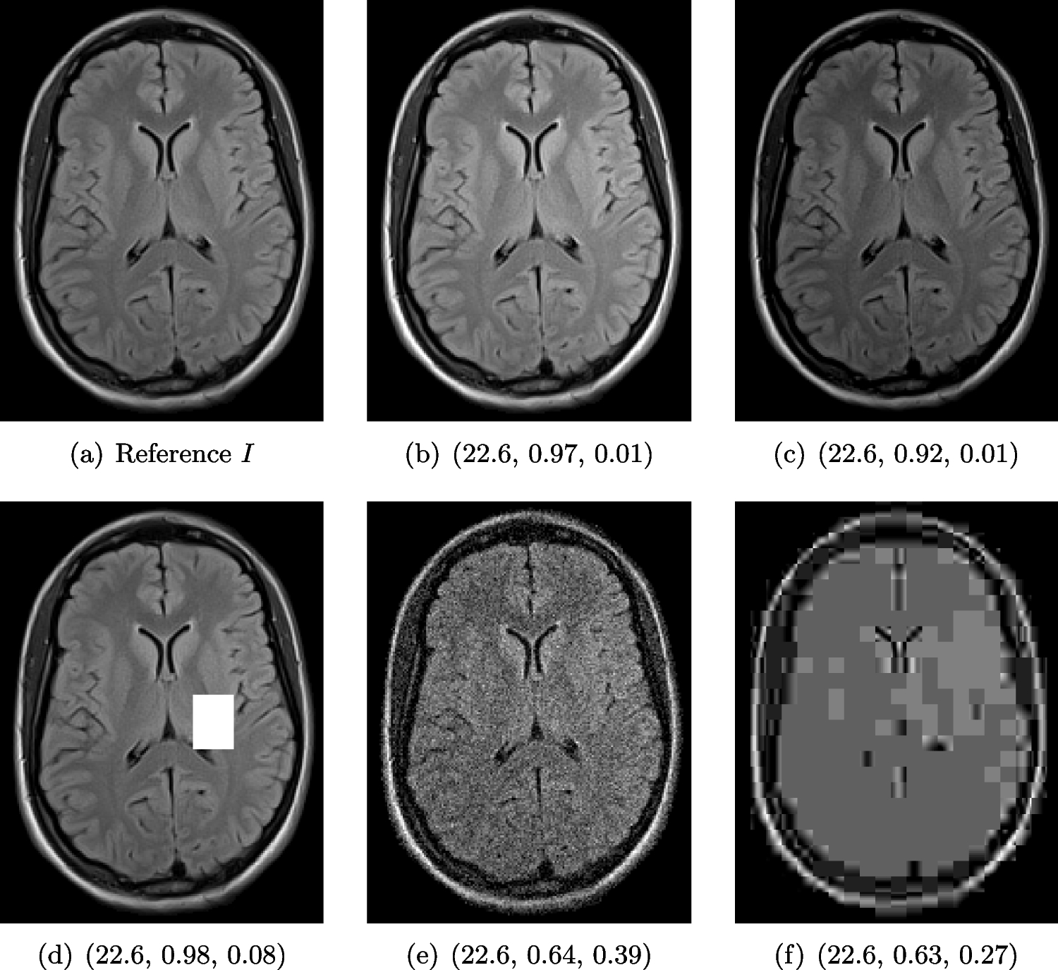
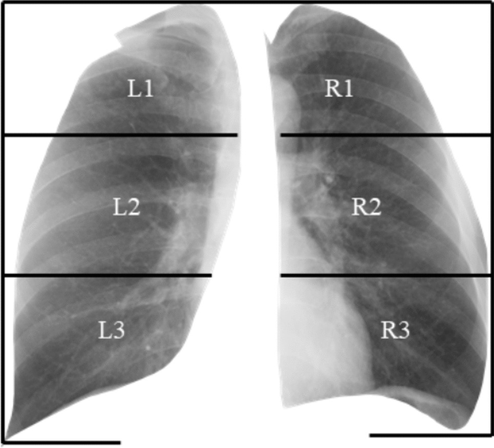
Chest X-ray scans with different kinds of post-processing: (a) serves as a reference, and (b) is wrongly judged as better visualization by PSNR/SSIM/LPIPS

FR-IQA Mismatch

We can see in Fig. 6 that PSNR and SSIM misjudge the visual quality of the high-resolution reconstruction in b in comparison to the up-sampled image in c. The image is per default more blurry and does not provide sufficient anatomical details and therefore offers worse visual quality than the reconstruction in b. LPIPS yields more sufficient results in this example and correctly attributes c a higher-quality error.

In this example, it has to be noted that the computed IQA numbers are generally quite low, because the resulting FA images do not necessarily have the same range or distribution as the reference image. Therefore, in order to compare the reconstruction quality directly, this task generally benefits from NR-IQA evaluation.

X-ray

X-ray imaging is a fundamental form of radiography. Reducing radiation dose while maintaining image quality is a key principle in radiology known as ALARA (as low as reasonably achievable) [84]. New technologies and imaging techniques, such as post-processing by artificial intelligence (AI) [43], may allow diagnostic objectives to be achieved with lower radiation doses. Furthermore, advancements in X-ray have also the potential to influence and enhance computed tomography (CT) [