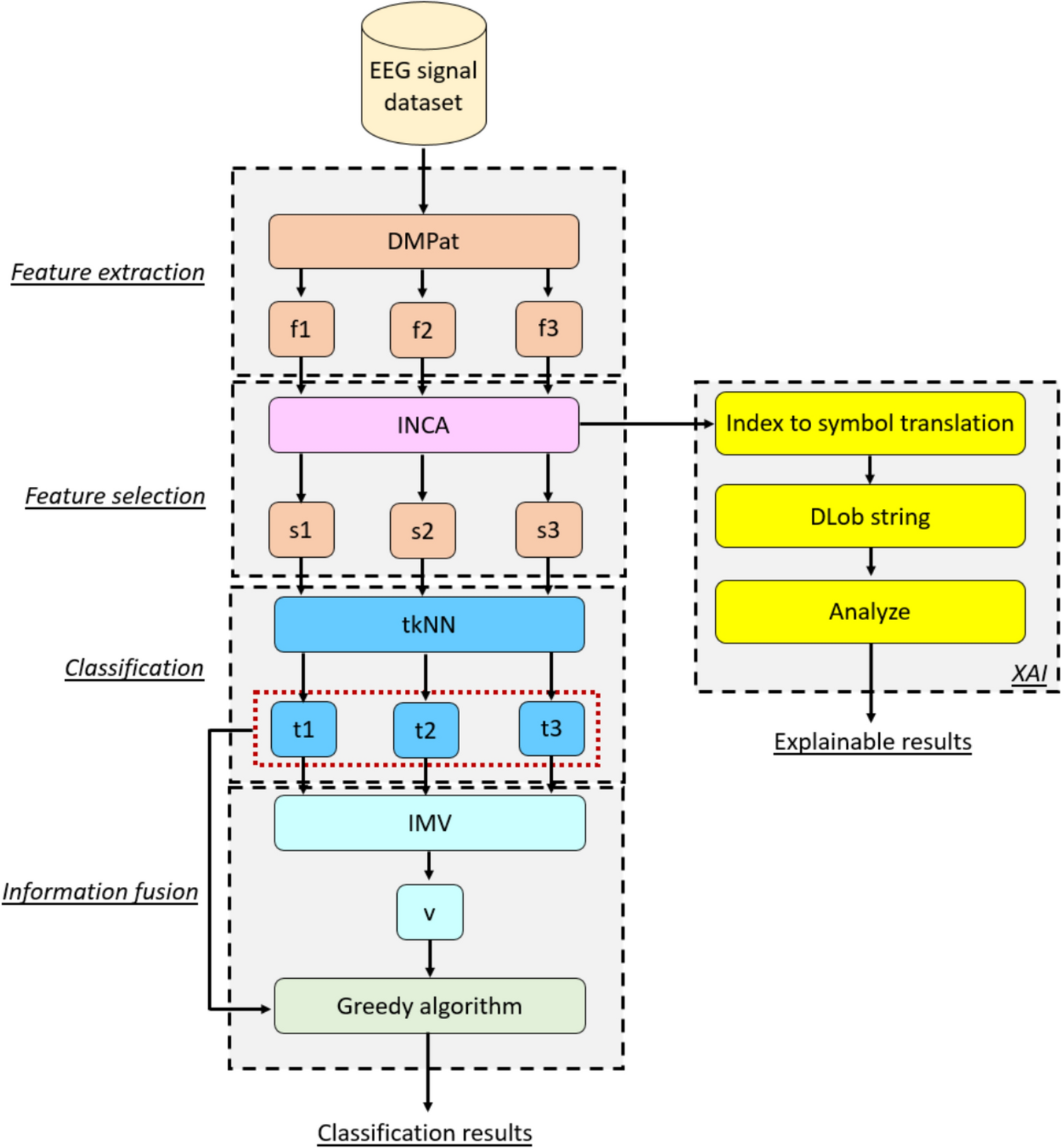
The essential objective of this SOXFE approach is to obtain high classification accuracy with explainable results. This approach has five main phases, which are:

DMPat-based FEX,

Feature selection based on INCA,

Explainable results employing DLob symbolic language,

tkNN-based classification,

Information fusion.

To clarify the presented approach, a visual depiction of this approach is showcased in Fig. 1.

Fig. 1

Visuıal overview of the proposed DMPat-based SOXFE approach. Herein, f: feature vector, s: chosen feature vector t: tkNN-based outcome and v: voted outcome

A detailed explanation of the recommended DMPat-based SOXFE approach is provided below.

Step 1: Apply DMPat to the proposed approach to extract features.

$$\left[_,_,_\right]=DMPat(EEG)$$

(1)

where \(DMPat(.)\): DMPat FEX function and \(f\): feature vector.

In this step, we derived three feature vectors, and the lengths of which are 196, 196, and 392, as the third feature vector is the concatenated version of the first two feature vectors. To better explain this step, the visual depiction of this feature vector is demonstrated in Fig. 2.

Fig. 2

Graphical explanation of the proposed DMPat FEX function

The steps of the presented DMPat are also given below for clarification.

Step 1.1: Create channel vector by reading channels of each point.

Step 1.2: Compute the distance vector for each channel value and create a distance vector.

$$DM\left(i,j\right)=\sqrt_^+C_^}, i,j\in \left\,\dots ,NC\right\}$$

(2)

Herein, \(DM\): distance matrix, \(NC\): number of channels and \(Ch\): channel value.

Step 1.3: Select the points with minimum and maximum distances.

$$\left[_,_\right]=argmin(DM)$$

(3)

$$\left[_,_\right]=argmax(DM)$$

(4)

Herein, \(a,b\): channels indices. By deploying these indices, feature map signals have been computed.

Step 1.4: Compute the feature map values deploying the extracted channel indices.

$$va_=_-1)\times NC+(_-1)$$

(5)

$$va_=_-1)\times NC+(_-1)$$

(6)

Herein, \(val\): the computed decimal values.

Step 1.5: Iterate steps 1.1–1.4 until the desired number of EEG signals is observed and value arrays are obtained.

Step 1.6: Extract histograms of the value arrays and obtain the first and second feature vectors.

$$_=\varepsilon \left(va_\right), k\in \\}$$

(7)

where \(f\): feature vector with a length of \(N^\), \(\varepsilon (.)\): histogram extraction function.

Step 1.7: Merge the first and second feature vector to generate third feature vector.

$$_\left(i\right)=_\left(i\right), i\in \,\dots ,N^\}$$

(8)

$$_\left(i+N^\right)=_\left(i\right)$$

(9)

These seven steps (Steps 1.1–1.7) have been defined in the presented DMPat.

In the presented DMPat, meaningful features are extracted. The use of minimum and maximum distances between EEG channels is based on the functional characteristics of brain activity. Minimum distances often indicate strong functional connectivity between adjacent regions, common during focused cognitive states or emotional processing. Although maximum distances show long-range interactions between distant brain areas. These distances show how different parts of the brain work together at a global level. By combining both local and distant relationships, the DMPat FEX method captures a broad range of inter-channel dynamics. Using this strategy, we can extract the meaningful features.

Step 2: Chose the most informative features by implementing the INCA feature selector, generate three selected feature vectors (Tuncer et al. 2020).

$$_=INCA\left(_,y\right),h\in \,3\}$$

(10)

Here, \(s\): selected feature vector, \(INCA(.)\): INCA feature selector, \(_\): hth feature vector and \(y\): actual/real labels.

The steps of the INCA feature selector appear as follows.

Step 2.1: Derive the qualified indexes by deploying NCA feature selector (Goldberger et al. 2004).

where \(id\): the qualified indexes of the by computing NCA feature selector.

Step 2.2: Deploy iterative feature selection.

$$s_^\left(d,j\right)=_\left(d,i_\left(j\right)\right), j\in \left\,\dots ,r\right\},$$

(12)

$$r\in \, d\in \,\dots ,nos\}$$

(L2)

Herein, \(sf\): iterative selected feature vector, \(start\): start index of the loop, \(stop\): stop index of the loop and \(nos\): number of segments.

Step 2.3: Derive the misclassification value of the selected features by deploying a classifier. In this research, we have used k-nearest neighbors (kNN) with tenfold CV.

$$loss\left(r-start+1\right)=}\left(s_^,y\right)$$

(13)

where \(loss\): the computed loss values and \(}(.)\): classifier.

Step 2.4: Select the best feature vector with minimum loss value. We employed a self-organized feature selector called INCA.

$$index=argmin(loss)$$

(14)

where \(^\): the ultimate selected feature vector of the hth method.

Step 3: Generate DLob string with the indices of the chosen features. The DLob string generation phase is demonstrated in below using mathematical equations (Tuncer et al. 2024a).

$$_=\lceil\frac_\left(t\right)}\rceil,t\in \,\dots ,N\}$$

(17)

$$_=sfi_\left(t\right) \left(mod NC\right)+1$$

(18)

$$dl_\left(c\right)=Table\left(_\right), c\in \,\dots ,2N-1\}$$

(19)

$$dl_\left(c+1\right)=Table\left(_\right)$$

(20)

Herein, \(Table\): look up table of the employed brain cap according to DLob, \(nid\): index of the DLob symbol, \(sfid:\) index of the chosen feature vector, \(N\): the number of the selected features, \(dls\): the generated DLob string. Moreover, the meaning of the used DLob symbols are given below.

FL: The left frontal lobe is referred to, being responsible for higher cognitive functions such as reasoning, decision-making, and problem-solving.

FR: The right frontal lobe is corresponded to, playing a key role in regulating emotions, social behavior, and understanding spatial relationships.

OL: The left occipital lobe is represented, being primarily involved in interpreting visual information from the right visual field.

OR: The right occipital lobe is stood for, processing visual stimuli from the left visual field.

PL: The left parietal lobe is signified, being responsible for integrating sensory information, spatial awareness, and aspects of language comprehension.

PR: The right parietal lobe is symbolized, being crucial for processing sensory inputs and contributing to spatial orientation and body coordination.

TL: The left temporal lobe is denoted, being essential for language comprehension, auditory processing, and memory functions.

TR: The right temporal lobe is represented, being associated with processing sounds, retrieving memories, and emotional responses.

We applied information entropy analysis, built transition tables for the cortical connectome diagram, and extracted insights from the three DLob strings.

Step 4: Assign classes to the chosen feature vectors via tkNN.

where \(t\): tkNN-based outcomes, \(^\): the ultimate selected feature vector of the hth method and \(y\): actual/real labels.

The tkNN is an ensemble classifier and the mathematical definition of classifier is given below (Tuncer et al. 2024a).

$$p_^=kNN\left(_,y,_,_,_\right),$$

(25)

$$a\in \left\,3\right\}, b\in \left\,\text\right\}, c\in \left\,\dots ,10\right\}, e\in \left\,\dots ,120\right\}$$

(26)

$$cac(e)=\phi \left(_^,y\right)$$

(27)

$$ix=argsort(-cac)$$

(28)

$$_^=\varpi \left(p_^, p_^,\dots ,p_^\right),l\in \left\,\dots ,118\right\}$$

(29)

$$cac(120+l)=\phi \left(_^,y\right)$$

(30)

$$_=\left\p_^, idx\le 120\\ v_^, idx>120\end\right.$$

(32)

Herein, \(dv\): distance value, \(w\): weight of the kNN, \(pout\): parameter-based outcome, \(cac\): classification accuracy, \(pout\): parameter-based outcome, \(\phi (.)\): classification accuracy computation function, \(ix\): the qualified classification accuracies by descending, \(vout\): voted outcome and \(idx\): the index of the maximum classification accuracy.

Equations (22)–(26) define the iterative parameter-based outcomes generation, Eqs. (27)–(29) explain the IMV algorithm, and Eqs. (30)–(32) represent the greedy algorithm. In this context, the tkNN used employs iterative parameter-based outcomes generation, IMV-based voted outcomes generation, and a greedy algorithm to choose the best outcome.

Step 5: Generate voted outcomes by deploying mode-based majority voting and select the best outcome via a greedy algorithm (DeVore and Temlyakov 1996).

$$vot=\varpi (_,_,_)$$

(33)

$$fot=GA(_,_,_,vot)$$

(34)

where \(vot\): the final voted outcome, \(fot\): the ultimate/final outcome and \(GA(.)\): greedy algorithm.

These five steps clearly defined the presented DMPat-based EEG VD approach. The graphical outcome of the tkNN classifier is demonstrated in Fig. 3.

Fig. 3

Graphical depiction of the tkNN classifier

The Fig. 3 shows the working of tkNN classifier. We generated voted outcomes by using the IMV and parameter-based outcomes. A greedy algorithm chosen the best result by choosing the outcome with the highest classification accuracy.