Sensors and ControllersLibelium e-Health Board

The e-Health board, made by Libelium, Fig. 3, is used to add the different types of sensors and capture the signals [19]. This board supports all the communication modules produced by Cooking Hacks, a brand that belongs to Libelium and oversees extending electronics to creators of all audiences in an accessible and educational way.

Fig. 3

If our board is too small for the dimensions of the project, layers can be added. The layers complement the functionality of the board model used, adding circuits, sensors, and external communication modules to the original board.

Microcontroller: Arduino UNO-R3

The Arduino UNO-R3 board, a versatile microcontroller powered by the ATmega328 chip, serves as the central hub for data acquisition and initial processing in this study, see Fig. 4. The choice of Arduino stems from its open-source nature, ease of programming, and vast community of support, making it an ideal platform for rapid prototyping and experimentation in the context of emotion recognition research. It has 14 digital input/output pins, 6 analog inputs, a ceramic resonator at 16 MHz, can be powered by battery or USB cable, and is programmed by computer. Communication between the two is through the serial port.

Fig. 4

Plan view of an Arduino UNO-R3 chip. Its components and its motherboard can be seen

Sensor Array

To capture nuanced physiological signals indicative of emotional states, a carefully curated array of non-invasive, cost-effective sensors forms the foundation of our data collection:

Pulse and Blood Oxygenation (SpO2): This sensor illuminates the skin with red and infrared light, measuring the differential absorption of oxygenated and deoxygenated hemoglobin. Variations in blood oxygenation levels reveal changes in heart rate and respiration, which are closely linked to emotional states.

Temperature: Body temperature fluctuations offer valuable insights into autonomic nervous system activity, which is highly responsive to emotional experiences. A dedicated temperature sensor continuously monitors the subject’s skin temperature.

Galvanic Skin Response (GSR): By measuring changes in the electrical conductivity of the skin, the GSR sensor provides a window into sweat gland activity regulated by the sympathetic nervous system. This offers a sensitive indicator of emotional arousal.

Airflow: This sensor measures breathing patterns, which can be used to detect changes in breathing rate and depth that are associated with emotional arousal.

The e-health board has several additional sensors, such as ECG, accelerometer, blood glucose, electromyogram (EMG), and blood pressure. However, these are not considered for several reasons. On the one hand, it has been observed that their value is not correlated with emotions in many cases, or they add too much noise, as in the case of the electromyogram. For this reason, it has been decided to adopt the simplest possible approach, seeking to increase the cost/benefit ratio.

The deliberate choice of this sensor suite prioritizes the following principles:

Non-invasiveness: User comfort and ease of deployment are prioritized by employing sensors that do not require complex procedures or direct penetration of the skin.

Cost-effectiveness: The selected sensors align with the study’s aim to develop an accessible emotion recognition system, making it feasible for broader applications.

Established Physiological Correlates: Each sensor targets well-understood physiological processes with documented links to the autonomic nervous system activity and emotional experiences.

Sensors are pre-calibrated according to the manufacturer’s specifications (see documentation [19])

Dataset

The database consists of 14 subjects aged between 25 and 67 years. The 5 physiological variables mentioned in the previous section (Sensor Array), i.e., pulse, oxygen, temperature, conductance, and airflow, were recorded during the measurement, all of which together with the date make up the database, which is anonymized to meet ethical and privacy criteria.

This measurement is recorded from a moment before the generation of the emotion, so first, we check that the sensors are giving normal values, then we introduce the stimulus that generates the emotion, in this case, a video of disgust or fear, and finally, we end the video and wait for the person to be stable again.

To facilitate the analysis of different emotional states, each measurement will be segmented into five stages that reflect the temporal dynamics of the emotional response:

Stage 1 (Baseline): Represents the initial stabilization period before stimulus presentation, capturing the subject’s resting physiological state.

Stage 2 (Pre-Emotion): Encompasses the period from the start of the stimulus until the onset of the target emotion (fear or disgust).

Stage 3 (Emotion): Marks the active experience of the target emotion, triggered by a specific event within the stimulus. It begins when an event of disgust or fear occurs.

Stage 4 (Post-Emotion): Captures the physiological changes as the subject transitions from the emotional state to its baseline.

Stage 5 (Recovery): Represents the return to the subject’s physiological baseline after the emotional experience.

This segmentation strategy allows for a nuanced analysis of the physiological patterns associated with each emotional stage. It will help identify which stages are most accurately classified by the artificial intelligence model and where potential challenges lie. For example, the similarity between Stage 1 (Baseline) and Stage 5 (Recovery) may pose difficulties for the system, but the crucial focus remains on the accurate identification of Stage 3 (Emotion). It has therefore been decided that, as they do not make a significant contribution to the results, stages 1 and 5 should be excluded to facilitate the reading and presentation of these results. Figure 5 depicts the stages of the data acquisition process.

Fig. 5

General data acquisition scheme

Selection of Subjects

Participants were selected randomly among volunteers to ensure that all subjects fell within a range of “normality.” All volunteers were screened by a psychologist to confirm that they were mentally healthy, as the study is not clinical, but aims to capture emotional responses only.

AI Algorithms

To construct the architecture of the emotion recognition model, a combination of CNNs, LSTMs, and attention layer was chosen among all the algorithms because it was the one that gave the best results when compared with other models.

CNN

A CNN is a deep learning architecture that is adept at image and video recognition, pattern analysis, and pixel-based data processing [20,21,22]. CNN’s use the convolutions to extract features from the input, see Fig. 6. Filters slide across the input image, performing element-wise multiplications and summations to generate feature maps (or activation maps). Through multiple layers of convolution and pooling, followed by fully connected layers, a CNN learns hierarchical representations—from simple edges and textures to complex objects and spatial patterns [23].

Fig. 6

Schematic of a CNN architecture with several convolutional layers similar to the one used in the model

The basic mathematical expression of a convolution operation in a CNN is as follows:

$$\left(f\ast g\right)\left(x\right)=\int_^\infty f\left(t\right)g\left(x-t\right)dt$$

(1)

where f is the input function, g is the kernel or filter that is applied to the input image, and x is the position in the image where the convolution operation is being performed. The above expression refers to convolution in one dimension, but in CNNs convolution operations are used in multiple dimensions, particularly in images that are two-dimensional matrices. This mathematical expression of a 2D layer in CNN is [24]:

$$}_}\text\left(_}^}_}^}_}^} \, \, }_}\text}_}\text}_}\right)$$

(2)

where:

O is the output tensor of dimensions (Io, Jo, K)

I is the input tensor of dimensions (Ii, Ji, C)

K is the kernel, or filter, tensor of convolution of dimensions (M, N, C, K)

f is the activation function. We chose ReLU because it introduces non-linearity into the network, which is essential for learning complex patterns in the data. Moreover, ReLU is computationally efficient and helps mitigate the vanishing gradient problem, thereby facilitating faster and more stable convergence during training.

b is the bias tensor.

The summation is over the indices m, n, and c to traverse the input tensor and the kernel tensor.

LSTM

Long-Short Term Memory Networks are a specialized variant of Recurrent Neural Networks (RNNs) designed to address the issue of vanishing gradients when handling long-term dependencies in sequential data. LSTMs achieve this through internal memory cells and gates that selectively regulate information flow, allowing them to retain and utilize contextually relevant information across extended time steps. This architecture has found success in domains such as speech recognition, natural language processing, and time series forecasting [25]. Variants like Bidirectional LSTMs (BiLSTMs) and Gated Recurrent Units (GRUs) offer additional refinements and capabilities.

The LSTM cell comprises a memory cell and three primary gates, which can be expressed mathematically as follows [26].

For our LSTM, assume that the hidden state \(}}_}-1}\) has dimension \(}\) and the input \(}}_}}\) has dimension \(}.\) Then, the weight matrices \(}}_}},}}_}}\), and \(}}_}}\) are of dimension \(}^}\times \boldsymbol\left(}+}\right)}\) and the corresponding bias vectors \(}}_}},\) \(}}_}},\) and \(}}_}}\) are in \(}^}}\).

Input Gate

This gate is responsible for updating the cell state using a sigmoidal activation function. It is defined as follows:

$$i_t\lbrack=\sigma(W_i.\left[h_,x_t\right]+b_i)$$

(3)

\(}}_}}\) is the weight matrix associated with the input gate of the LSTM. It is used to map the concatenated vector \([}}_}-1},\boldsymbol}}_}}]\) (which combines the previous hidden state and the current input) into the cell state space.

\(b_i\in\mathbb^d\) is the corresponding bias vector.

\(}}_}}\) is the input vector at the current time step. It contains the features or measurements from the system at time \(t\) and has a dimension \(}.\)

\(}}_}-1}\) represents the hidden state from the previous time step in the LSTM. It contains the information that was computed up to time \(}-1\) and is used, together with the current input \(}}_}\), to determine the operations of the LSTM’s gates and to update the cell state.

σ denotes the sigmoid function, which outputs values in the interval [0,1] to determine the proportion of new information to be retained [25, 26].

Forget Gate

This gate decides which information should be discarded from the cell state. It is expressed as:

$$f_t=\sigma(W_f.\left[h_,x_t\right]+b_f)$$

(4)

 where \(_\in\mathbb^and\;_\in\mathbb^\) serve similar roles for the forget gate (weight representation and bias).

Output Gate

This gate determines the output of the LSTM cell based on a filtered version of the cell state [26]. It is computed as follows:

$$o_t=\sigma(W_o.\left[h_,x_t\right]+b_o)$$

(5)

Here, \(_\in\mathbb^and\;_0\in\mathbb^\) are the weight matrix and bias for the output gate. The \(tanh\) function compresses the cell state \(_\) into the range [− 1,1] for output generation.

Cell State Update

Finally, the previous cell state \(_\) must be updated as follows. The complete process can be seen in Fig. 7.

$$C_t=f_t.C_+i_t.g_t$$

(7)

where \(_=tanh(_\cdot [_,\hspace_]+_)g\_t\) represents the candidate cell state computed using the hyperbolic tangent function \((tanh)\), with \(}}_}}\) \(\in\mathbb^\) and \(}}_}}\) \(\in\) \(}^}}\).

Fig. 7

Scheme of the components of a LSTM cell

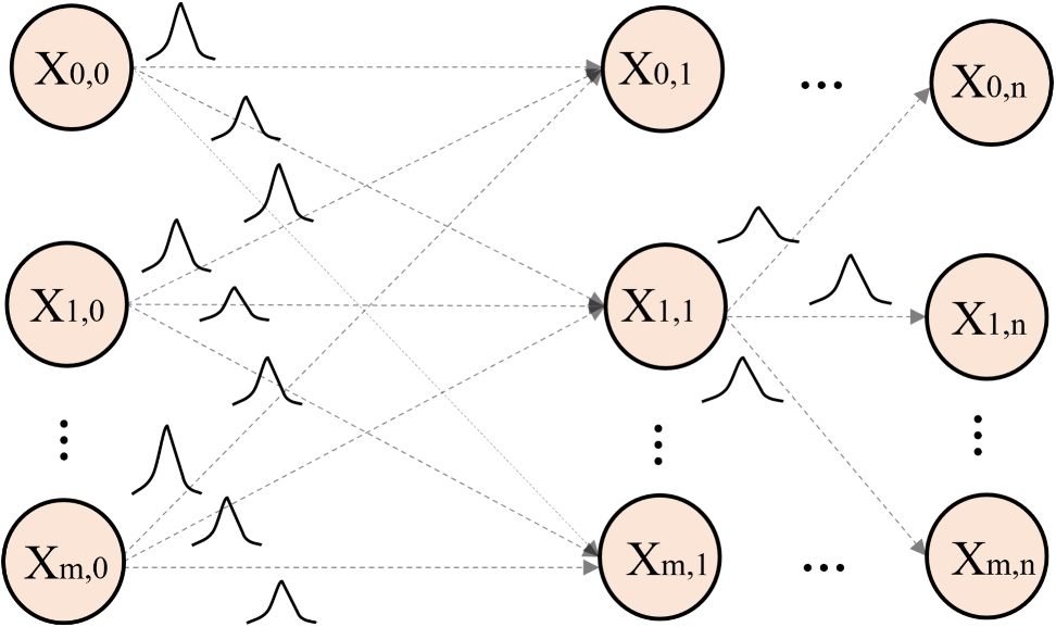
Attention Layer

The attention layer is a fundamental component in deep neural network architectures, especially for tasks involving sequence processing such as machine translation, text summarization, and speech recognition. Its main function is to focus the model’s attention on the most relevant parts of the input in order to produce an accurate output.

An attention layer takes as input a sequence of vectors h1, h2, …, hn and produces a sequence of attention vectors a1, a2, …, an, where each ai represents the relative importance of hi in the final output, see Fig. 8.

Fig. 8

Scheme of a multi-head attention layer

The attention vectors are computed using a scoring mechanism that assigns a score to each input vector. The scoring function can be as simple as a dot product or as complex as a deep neural network [27].

Where X is the data matrix, Q, K, and V are the subnetworks of the attention head, w indicates that the subnetworks are weighted and, finally, after the dot products, a concatenation is performed using softmax to output a linear vector.

Important Additional Layers

It is necessary to add other types of layers to optimize the procedure and also for the model to work correctly, the most important ones are as follows:

Dense Layer

A dense or fully connected layer establishes connections between every neuron in that layer and every neuron in the subsequent layer. This structure is essential for learning complex relationships within data. The mathematical representation for a simple fully connected network with one hidden layer and an output layer is [28]:

$$y_=f\left(^n}(W_i\ast x_i)+b\right)$$

(8)

where:

\(}}_}}\) is the input vector to the network.

\(}}_}}\) are the weight matrices for the connections between layers.

\(}\) is the bias.

\(}\) is the activation function applied to the output of each layer to compute the attention weights. The election was the softmax function. This choice ensures that the weights are normalized into a probability distribution across the input sequence, allowing the model to focus more on the most relevant features.

Note that deep neural networks often contain multiple hidden layers, leading to more intricate formulas with additional weight matrices and bias vectors.

Dropout layer

Dropout is a regularization technique designed to mitigate overfitting in deep learning models. During training, it randomly deactivates (sets to zero) a specified percentage of neurons at each iteration. Mathematically, a dropout layer multiplies the input vector by a randomly generated binary mask with the exact dimensions. The probability that a mask element is 1 is termed the “dropout rate” (commonly between 0.2 and 0.5).

Note that dropout is typically deactivated during testing (dropout rate set to 0), and dropout rates depend on the model’s complexity and the dataset [29].

Hyperparameters

Fine-tuning the hyperparameters is essential to optimize performance and prevent overfitting or underfitting. Here are shown the most important used in the model:

Optimizer: Adam is a popular optimization algorithm that combines the strengths of RMSprop and Momentum. It computes adaptive learning rates for each parameter based on estimates of first and second moments of the gradients. The following Eqs. (9–11) describe the Adam optimizer [30, 31]:

$$m_t_1m_+\left(1-\beta_1\right)g_t$$

(9)

$$v_t=\beta_2v_+\left(1-\beta_2\right)g_t^2$$

(10)

$$\theta_t=\theta_-\frac\alpha+\epsilon}m_t$$

(11)

where:

\(}}_}}\) is the first updated moment (mean) estimate.

\(}}_}}\) is the second updated moment (variance) estimate.

\(}}_\) and \(}}_\) are the moment decay parameters.

\(}}_}}\) is the gradient at the current step.

α is the learning rate.

ϵ (epsilon) is a small numerical constant to avoid division by zero.

\(}}_}}\) is the current value of the parameter being updated. This is the parameter that the algorithm optimizes.

Adam was selected due to its robustness in handling sparse gradients and its proven performance across various deep learning tasks [30, 31].

Learning Rate: \(1\times ^\)

The learning rate controls the magnitude of parameter updates during training. The choice of a learning rate of \(1\times ^\) is based on preliminary experiments and supported by prior literature, ensuring stable convergence without overshooting minima.

Batch Size: 5, 10 and 15

The batch size defines the number of examples processed per iteration. We evaluated different batch sizes and found that a batch size 15 offered a good balance between computational efficiency and convergence behavior. Larger batch sizes generally improved gradient stability, but we observed diminishing returns beyond a batch size of 15 in our experiments.

Epochs: 1000

The number of epochs represents the number of complete passes through the training dataset. An epoch count of 1000 was determined to be sufficient to allow the model to learn the underlying patterns in the data, with early stopping applied based on validation performance.

Momentum: 0.99 and 0.999

Momentum values were employed to control the influence of previous updates on new ones. These values help accelerate gradient descent in the relevant direction and dampen oscillations, contributing to faster convergence.

Shuffling:

Shuffling the training data at each epoch is applied to ensure a random distribution of examples, which helps prevent the model from learning the order of the data.

Activation Function: ReLU

As it was explained in section 2.3.1. ReLu was used in the CNN layers due to its ability to introduce non-linearity, facilitate efficient gradient propagation, and mitigate the vanishing gradient problem.

Regularization: (rate 0.2 to 0.5)

Dropout is a regularization technique where a fraction of neurons is randomly deactivated during training. This helps prevent overfitting by ensuring that the model does not rely too heavily on any single feature

The selection of these values was based on prior literature and experimentation with different configurations. Finding the optimal hyperparameter configuration is an iterative process that requires careful testing and adjustments.

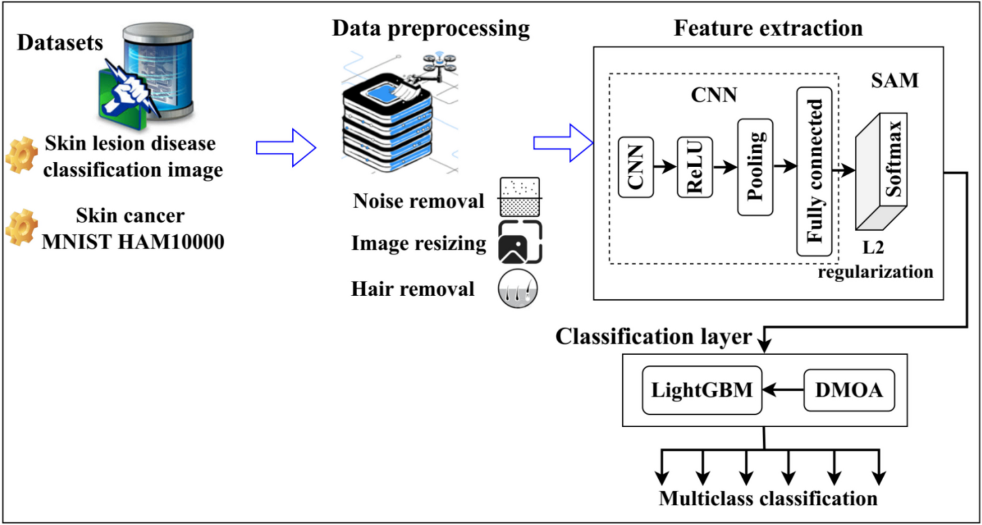
Architecture of the Network

The diagram that is shown in Fig. 9 shows a system that uses sensors to capture the emotional responses during video viewing. The captured signal is vectorized and normalized using the Z-score function, resulting in 1D vectors of dimension (19,1,1). These overlapped vectors, encompassing multiple events, are fed into a 3-layer 1D CNN with feature maps of decreasing size (128, 64, 32) for efficient feature extraction.

Fig. 9

Architecture of the network

The output then passes through a fully connected layer with a single output neuron, followed by a dropout layer to reduce overfitting. The resulting vector is flattened and then processed through sequential LSTMs, each containing 64 neurons, to capture temporal dependencies within the emotional response. Finally, the output of the LSTM layer is passed through an attention layer to focus on the most relevant features before final classification through a softmax layer.

Performance Indices

This study employs a set of widely accepted metrics in the literature to validate the obtained results [32,33,34]:

Accuracy: It measures the overall correctness of the model’s predictions, calculated as the ratio of true positives and true negatives to the total number of samples.

Precision: It reflects the proportion of positive predictions that are correct, calculated as the ratio of true positives to the sum of true positives and false positives.

Recall (Sensitivity): It quantifies the model’s ability to identify all positive instances, calculated as the ratio of true positives to the sum of true positives and false negatives.

F1 Score: It provides a weighted average of precision and recall, offering a more balanced assessment of the model's performance, calculated as 2 * (precision * recall)/(precision + recall).

$$F1=2.(Precision\ast Recall)/(Precision+Recall)$$

(13)

Specificity: It measures the model’s ability to correctly identify negative instances, calculated as the ratio of true negatives to the sum of true negatives and false positives.

where TP are true positives, FP are false positives, TN are true negatives, and FN are false negatives.

Confidence interval (CI): is an estimated range of values, derived from sample data, that is likely to contain the true value of a parameter (such as the model’s accuracy) 95% of the time. The CI provides insight into the precision and reliability of the estimate. We use the binomial proportion approach [35].

$$CI=\widehat p\pm Z\alpha/2\sqrtn}$$

(15)

where \(\widehat}}\) is the observed accuracy, \(}\) is the total number of samples, and \(}_^}\!\left/ \!_\right.}\) is the critical value from the standard normal distribution (e.g., 1.96 for a 95% CI). Although the Clopper–Pearson exact interval [36] can also be used for smaller sample sizes, the normal approximation typically suffices for moderately large \(}\). This confidence interval helps assess the robustness of our accuracy estimate by providing a plausible range of values.

p-value: represents the probability of observing the given results, or something more extreme, under the assumption that the null hypothesis is true. In the context of our model, it quantifies the likelihood that the observed accuracy (e.g., 93.75%) could have occurred by random chance if the true accuracy were at a baseline level (typically 50% for binary classification). A small p‐value (commonly < 0.05) indicates that such an outcome is highly unlikely under the null hypothesis, thus suggesting that our model’s performance is statistically significant [37].

To determine whether the observed accuracy significantly exceeds chance (50% for random binary classification), a one‐sided binomial test is performed [38, 39]. Under the null hypothesis \(}}_:}=0.5\), the probability of obtaining \(}\) or more correct predictions out of \(}\) is:

$$}-}}}}}=\sum_}=}}^}}\left(\begin}\\ }\end\right)\right)}^}}$$

(16)

where \(}\) is the total number of predictions (or observations), \(}\) is the number of successes observed, and \(\left(\begin}\\ }\end\right)\) is the binomial coefficient which represents the number of ways to choose \(}\) successes out of \(}\) trials.

These definitions help ensure that our reported performance metrics are both precise (through the CI) and statistically validated (through the p‐value).

Hardware and Time Computing.

The present work was developed on a hardware with the following specifications; CPU i7-9700 K, 16 Gb RAM-DDR4, Nvidia RTX-2060 Super Windforce OC (8 VRAM). The computation time for training and test was 85.16 ± 2.065 s and 0.01165 ± 0.004 s (11 ms approx.).