
Remember me
This study was approved by the Institutional Animal Care and Use Committee of Tohoku University and performed in accordance with published guidelines.
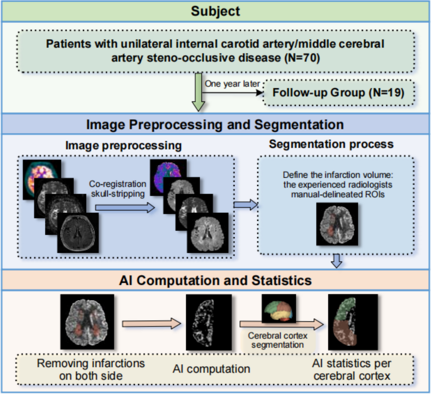
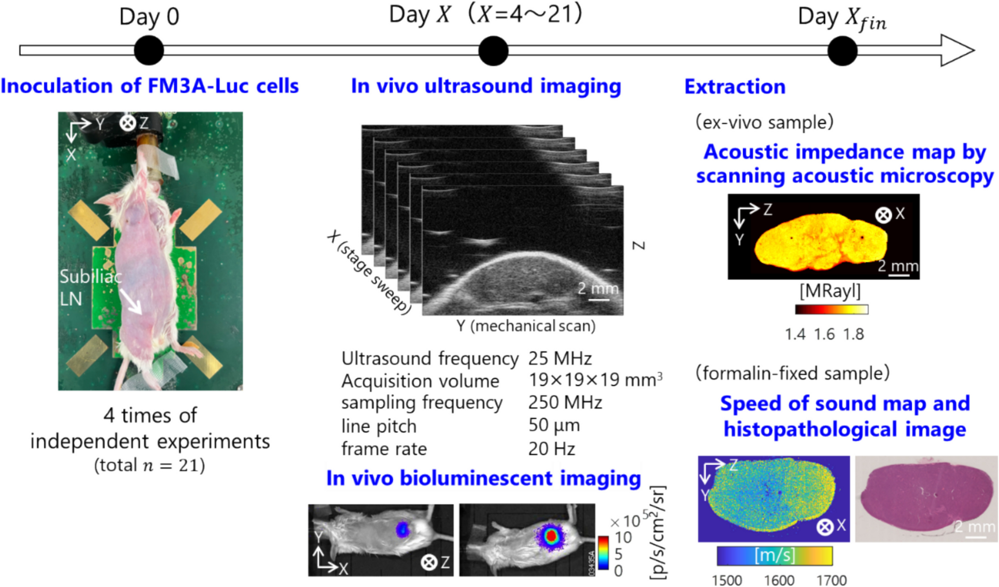
The overview of this study design is shown in Fig. 1. The subiliac LN (SiLN) of MXH10/Mo/lpr mouse was used as a pseudo-sentinel LN by inoculating it with a tumor. We used FM3 A-Luc cells, mouse mammary carcinoma cells, that constitutively express the luciferase gene as followed in our previous study [36]. The culture medium for FM3 A-Luc cells consisted of RPMI (Sigma-Aldrich) containing 10% fetal bovine serum, 1% L-Glutamine-P.S. Solution, and 0.5% Geneticin (G418, Sigma-Aldrich). The cell suspension was further diluted threefold with Matrigel, resulting in a final cell concentration of 3.3 × 10⁵ cells/mL. For the inoculation, mice were anesthetized with 2% isoflurane in air, and 60 µL of the cell suspension was directly bolus injected into the SiLN by a 27G Nipro Myjector syringe. (Figure 2)
Fig. 1.
Schematic image of study design
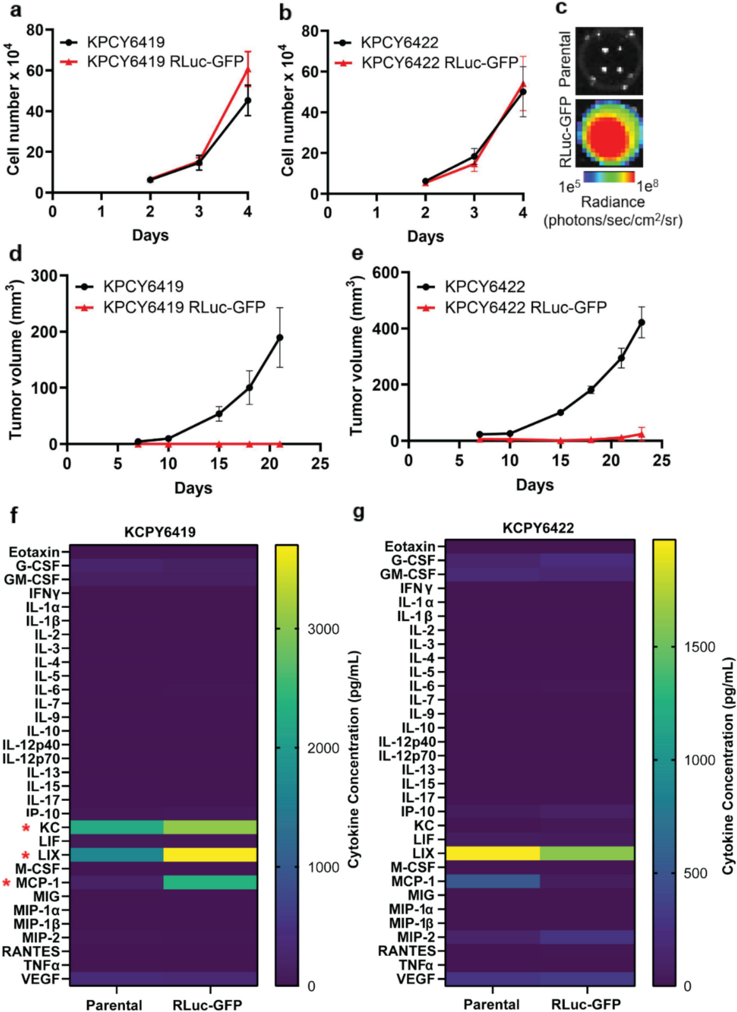
Fig. 2.
Schematic image of ultrasonic attenuation estimation
In Vivo MeasurementUltrasonic measurement and bioluminescence imaging were conducted on the following day in each experiment: Group I (\(n\)= 4) on days 0, 7, 14, and 21 with the day of tumor cell inoculation designated as day 0. For the reproducibility of this study, the additional data collection was performed on Group II (\(n\) = 5) on days 0, 4, 6, 8, and 11; and Group III (\(n\)= 5) on days 0, 4, 7, 10, 13, 16, and 20; Group IV (\(n\) = 7) on days 0, 7, 10, 13, and 16.
To evaluate tumor growth, we used a bioluminescence imaging system (IVIS Lumina LT series III, Perkin Elmer). Mice were anesthetized with 2% isoflurane, and 15 mg/mL luciferin (D-Luciferin Potassium Salt, FUJIFILM Wako) was injected intraperitoneally. Bioluminescence intensity was measured 10 min later. The average luminescence [10 log10(intensity)] per unit time was calculated using the accompanying analysis software (Living Image, Perkin Elmer).
The mouse was also anesthetized and positioned on a heated stage for in vivo ultrasound imaging. The ultrasound scanner (Vevo 770, FujiFilm) with a mechanical single-element transducer (RMV- 710B, VisualSonics, FujiFilm) was used to observe LN and collect A/D converted data. The center frequency of the single-element transducer is 25 MHz. The pitch of scanline imaging is 0.05 mm. A laboratory-made data acquisition system for radio-frequency (RF) signals was constructed using a Vevo 770 and an A/D board (Sbench 6, Spectrum) with a sampling frequency of 250 MHz and 14-bit digitization. A single-element transducer was mechanically scanned across Y-axis of 19 mm (380 pixels) and X-axis of 19 mm (190 pixels) using a motorized stage synchronized with the A/D board. The frame rate was 20 fps. The acquired time for data curation was around 10 s. Three-dimensional reconstructed RF data was used to estimate the local AC.
Ex Vivo MeasurementAfter a sacrifice on the final day of in vivo measurement, the SiLN was extracted for acoustic characterization. The cross-section at the maximum surface of the LN was divided as raw (for acoustic impedance) and formalin fix samples (for SAM and histopathology).
For the comprehension of acoustic impedance in microscopic structure, RF data (8 bits and 2 GS/s sampling frequency) were measured from ex vivo tissue cross-sections via distilled water on a polystyrene dish by a 80 MHz single-element transducer (HD80–1.2–2.5, Toray). The data acquisition system was modified SAM (modified AMS- 50 SI, Honda Electronics). There is a limitation that the scanning area was 4.8 mm × 4.8 mm (scanning pitch of 16 μm) at the maximum. Hence, the scanning area was readjusted to two dimensions (2D) to observe the whole spatial distribution in the cross-sections of the LN. All acquisition protocols were followed by the previous study [37] using commercial software (UMScope, Honda Electronics). The acoustic impedance was analyzed using the reference medium theory [38].
After formalin fixation of the ex vivo LN, the samples were embedded in paraffin and sectioned into continuous 7 μm thick slices for SoS analysis and pathological observation. The dataset for SoS analysis was acquired using a laboratory-made scanner [39] with a 300 MHz single-element transducer (HT- 400 C, Honda Electronics). Briefly, RF signals from a sliced specimen via distilled water on a glass plate were obtained through 2D scanning of the entire lymph node region, with a sampling frequency of 2.5 GHz and 12-bit digitization. The SoS was calculated by the time-of-flight of RF signals separated by an autoregressive model [40]. The pathological specimens were stained using the hematoxylin–eosin method and observed with a virtual slide scanner (NanoZoomer S60, Hamamatsu Photonics) equipped with a 40 × magnification lens.
Attenuation EstimationThe local AC was computed using the log-difference method using reference phantom [41, 42]. The local window with the size of 1.0 mm2 [336 (in Z-axis) × 20 (in Y-axis)] pixels] was scanned within the internal LN. To consider the motion artifact due to cardiac beat, the scanning frame in the presence of displacement was eliminated to estimate the local AC. The LN region was initially grouped by superpixels [43] and segmented by k-means method [44] into background, skin, and internal LN.
The power spectrum \(P\) of the backscattered signal can be defined by the system's transmission-reception characteristics \(S\), \(BSC\), and the attenuation characteristic of the exponential term as \(P\left(f\right)=S\left(f\right)\bullet BSC\left(f\right)\bullet ^\). When taking the natural logarithm of the equation, it can be defined as \(\text\left[P\left(f\right)\right]=S\left(f\right)+BSC\left(f\right)-4\alpha df\). Considering the frequency characteristics of the backscattered waves in the LN, \(_\) relative to the reference one \(_\) at arbitrary depths \(_\) and \(_\),
$$\left.\text\left(\frac_\left(d,f\right)}_\left(d,f\right)}\right)\right|_=4_-_)_f+\Delta BSC(f)$$
(1)
$$\left.\text\left(\frac_\left(d,f\right)}_\left(d,f\right)}\right)\right|_=4_-_)_f+\Delta BSC(f)$$
(2)
Here, assuming that the BSC is constant at \(_\) and \(_\), solving from Eqs. (1) and (2), we obtain
$$_f=8.686\frac\left(\frac_\left(d,f\right)}_\left(d,f\right)}\right)\right|_-\left.\text\left(\frac_\left(d,f\right)}_\left(d,f\right)}\right)\right|_}_-_\right)}+_f$$
(3)
The equation allows for the calculation of the frequency dependence of the attenuation as described below. Furthermore, by performing a linear approximation of the attenuation obtained from Eq. (3), the slope can be derived as the AC \(_\). The useful frequency range was 6–31 MHz at \(-\) 20 dB bandwidth. The AC \(_\) of reference phantom was 0.22 dB/cm/MHz in the total attenuation estimation using the reflector method [45]. The distance between \(_\) and \(_\) was 2.5 mm to include the whole region of the LN.
Acoustic Characterization with Acoustic Impedance and Speed of SoundSecondly, for the comprehension of the acoustic property and histopathology, we spatially compared acoustic impedance, SoS, and pathological images. The acoustic impedance \(_\) was calculated from both the reference RF signal (negative-peak voltages \(_\)) with known acoustic impedance (\(_\) and \(_\)), and the sample signal \(_\) from the cross-sectional sample [38] as follows
$$_=\frac_}_}\frac_-_}_+_}\right)}_}_}\frac_-_}_+_}\right)}_$$
(4)
The acoustic impedance of the purified water, \(_\), and that of the polystyrene dish, \(_\), were set at 1.50 and 2.35 MRayl, respectively [38].
The RF data from the specimen for SoS analysis was firstly separated with two signals: distilled water – surface of the specimen (first wave) and bottom of specimen – glass plate (second wave) using a fifth-order autoregressive mode model [39]. The time-of-flight between specimen and reference (i.e., distilled water – glass plate signals without specimen) data was calculated by
$$_=\frac_}_-\Delta _}_,$$
(5)
where \(\Delta _\) and \(\Delta _\) represent the time-of-flight between the first and reference waves, and the second and reference waves, respectively.
Comments (0)