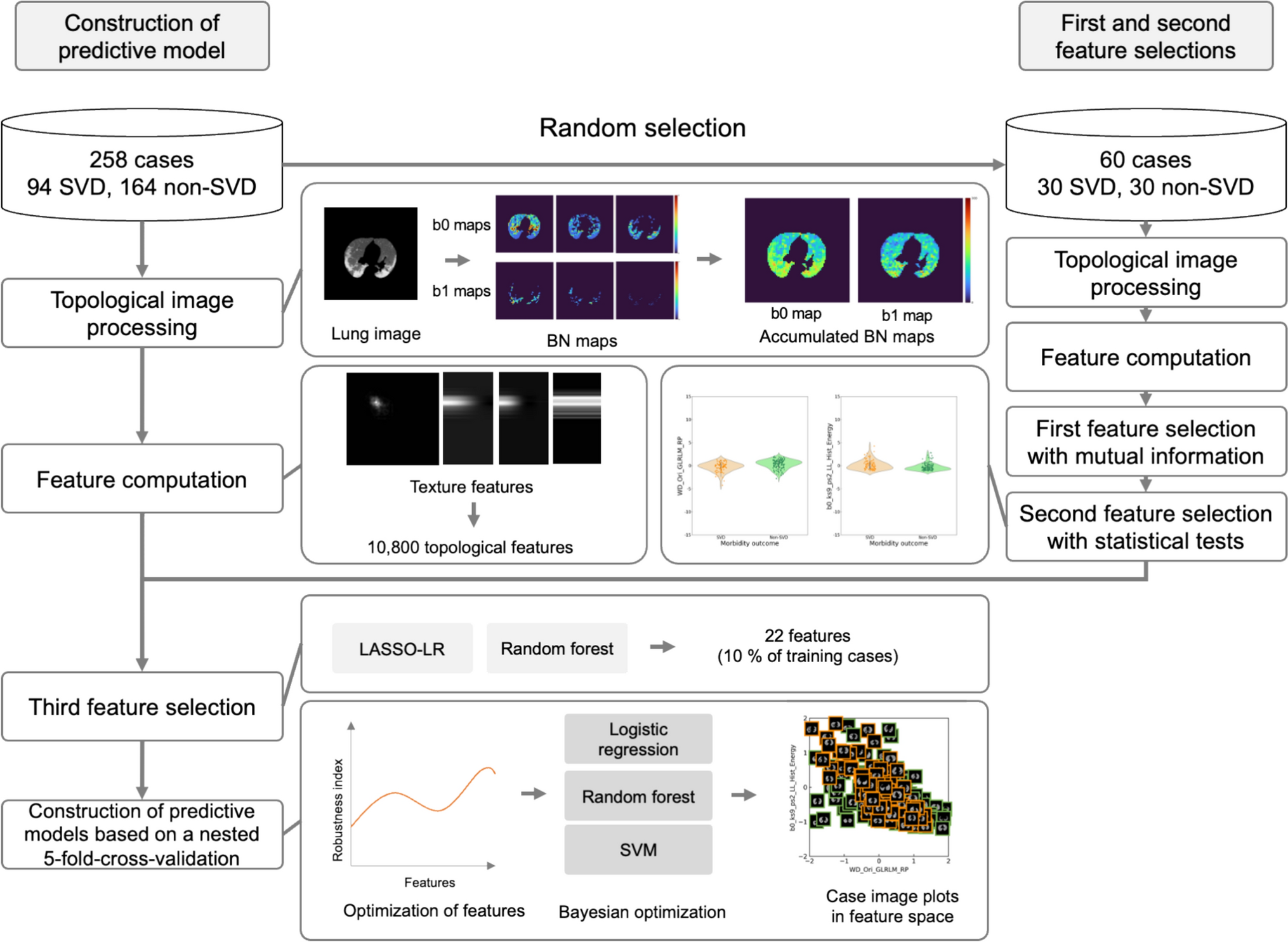
Table 1 summarizes the patient information used in this study. The CT images of 258 patients with COVID-19, consisting of 94 SVD and 164 non-SVD patients, were collected from an open database provided by Huazhong University of Science and Technology [18]. All patients underwent RT-PCR and CT scanning at the Union Hospital (China) and the Liyuan Hospital (China). The pneumonia regions were segmented using Otsu’s automatic thresholding technique [25], because it is difficult to determine the precise pneumonia region in clinical situations.

Table 2 shows the patient information of 60 cases with annotated pneumonia regions for the first and second feature selections. Sixty patients, consisting of 30 SVD and 30 non-SVD patients, were randomly selected from the 258 patients. The pneumonia regions were segmented using Otsu’s automatic thresholding technique [25] and manually corrected using a 3D slicer [26]. A radiologist (S.I.) validated the pneumonia regions. The 60 patients were included in the training data.

The patients were scanned on various CT scanners [TOSHIBA (Japan), SIEMENS (Germany), PHILIPS (Netherlands), and United Imaging Healthcare (China)] with voltages of 100 or 120 kV, pixel sizes of 0.633 mm2 to 0.977 mm2, slice thicknesses of 1.5 mm–2.0 mm, and a matrix size of 512 × 512. A single slice containing the pneumonia region was selected for each patient.

Figure 1 shows the overall workflow for constructing a predictive model of SVD in patients with COVID-19 pneumonia using accumulated BN maps. A total of 258 patients were randomly divided into 198 patients for model construction and 60 patients for first and second feature selections. BN maps were generated in topological image processing by calculating BNs (b0 and b1) within a shifting kernel in a manner similar to a convolution. BN maps derived from a range of threshold values were accumulated for each BN map for topological feature computation. In the first and second feature selections, significant feature candidates were selected from the features computed in the pneumonia regions of 60 cases based on the p values of statistical tests following mutual information between SVD and non-SVD patients. Subsequently, two feature selection methods were deployed for the third feature selection. Predictive models of SVD were constructed using nested fivefold cross-validation (CV) encompassing the training and test datasets, as shown in Supplementary Fig. 1 (Online Resource 1). The nested fivefold CV was leveraged to estimate unbiased results and reduce the chance of information leakage which could make our models stable and reproducible [27,28,29]. In the fivefold nested CV, the numbers of training and test cases were 208 or 206 (76 or 75 SVD, 131 or 132 non-SVD) and 50 or 52 (18 or 19 SVD, 32 or 33 non-SVD), respectively, depending on the fold.

Overall workflow for constructing a predictive model of SVD in patients with COVID-19 pneumonia using accumulated BN maps

94 SVD patients and 164 non-SVD patients were used to construct accumulated BN maps within lung regions. The lung regions were segmented using Otsu’s automatic thresholding technique [25]. Lung images were obtained by cropping the lung regions from the original CT images. The lung images were transformed into isotropic images with a pixel size of 0.98 × 0.98 mm2 using cubic and shape-based interpolations [30], during which the gray-scale values from -1350 to 150 Hounsfield units were normalized to 0 to 255 scale to suppress pixel value variations.

Following the preprocessing, the lung images were consecutively binarized by multiple-threshold values to calculate the corresponding BN maps, followed by the accumulation of BN maps. Figure 2 illustrates the calculation of b0 and b1 maps in a binary image obtained from a lung image. The b0 and b1 were computed within a square kernel, and then, those values were placed at a pixel corresponding to the center pixel of the kernel in a manner similar to a mathematical convolution. The resultant images of b0 and b1 were referred to as b0 and b1 maps, respectively, which indicate the topological properties as color maps. The b0 and b1 maps represent maps of the numbers of connected and hole components, respectively.

Calculation of b0 and b1 maps in a binary image obtained from a lung image. A pneumonia region is shown by yellow line. The kernel with a size of 5 pixels and shifting pixel of 5 were utilized for this case. In enlarged area (enclosed by red line), white areas represent the connected components and black areas represent the hole. Since b0 represents the number of connected components (white area), the number of connected components is one, which means b0 = 1. b1 represents the number of holes (black area) and there are two black area enclosed by white area, which means b1 = 2. Color bars indicate the Betti number from dark blue to dark red corresponding to 0 to higher numbers

Figure 3 shows an original image, binary images consecutively binarized by multiple-threshold values from 50 to 255 with increments of 1, and their corresponding b0 and b1 maps. The accumulated BN maps are shown in the last column. The method for determining the initial threshold value for accumulated BN maps is described in Online Resource 2. For each binary image, b0 and b1 were computed within a square kernel, as shown in Fig. 2.

An original image, binary images consecutively binarized by multiple-threshold values from 50 to 255 with increments of 1, and their corresponding b0 and b1 maps. The accumulated Betti number (BN) maps are shown in the last column. The kernel with a size of 5 and shifting pixel of 5 were utilized for this case. Color bars indicate the BNs or accumulated BNs from dark blue to dark red corresponding to 0 to higher numbers

All b0 and b1 maps generated with the same kernel size and shifting pixel were summed to construct the accumulated b0 and b1 maps over consecutive threshold values from 50 to 255, as shown in Fig. 3. The kernel sizes of 5, 7, 9, and 11 pixels and shifting pixels of 1, 2, 3, 4, and 5 pixels were applied to the construction of the accumulated BN maps [12].

A total of 10,800 topological features were obtained for each patient from 270 radiomic features × 2 accumulated BN maps (b0 and b1) × 4 kernel sizes × 5 shifting pixels. The radiomic features were composed of 14 histogram and 40 texture features in 5 types of images [an original accumulated BN map and four wavelet-decomposed (WD) images]. Gray-level co-occurrence matrix (GLCM), gray-level run-length matrix (GLRLM), gray-level size zone matrix (GLSZM), and neighborhood gray-tone difference matrix (NGTDM) were used to extract texture features. Wavelet decomposition was applied to the accumulated BN maps to obtain four WD images using the high (H)-pass filter and low (L)-pass filter based on the coiflet1 mother function [LL, LH, HL, and HH (each of the characters, L or H, represents a low-pass or high-pass filter, respectively)]. The topological features were corrected using harmonization [31,32,33]. In addition, topological features were augmented using the Synthetic Minority Over-sampling Technique (SMOTE) to improve the stability of predictive models with a small dataset. These features were then standardized to z-scores by the training dataset in every outer loop of the nested fivefold CV [34]. The feature computation was performed using a MATLAB-based radiomics tool package (MATLAB 2024a, MathWorks) [35].

The significant features were selected in three steps. In the first feature selection, significant feature candidates were selected from the features computed in the pneumonia regions of 60 cases (Table 2) based on mutual information between SVD and non-SVD patients. Figure 4 depicts the pneumonia regions on the original CT images for an SVD patient and a non-SVD patient and their corresponding accumulated BN maps with contours of the pneumonia regions. After computing the topological features of 30 SVD patients and 30 non-SVD patients, the number of features was decreased using mutual information to 108 (1.0% of 10,800) [36]. In the second feature selection, statistical tests between SVD and non-SVD patients were performed. The significance level was set at p < 0.05. The normality of the features was validated using Shapiro–Wilk test. When p values were lower than 0.05, Mann–Whitney’s U tests were applied to the features. When p values were 0.05 or more, an analysis of variance was performed. Welch’s t tests were applied to the features with p values lower than 0.05, whereas Student’s t tests were applied to the other features. The p values were corrected using the false discovery rate (FDR) to account for multiple comparisons [37].

Pneumonia regions on original CT images for an SVD patient and a non-SVD patient and their corresponding accumulated BN maps with contours of the pneumonia regions. Color bars indicate the accumulated BNs from dark blue to dark red corresponding to 0 to higher numbers

Two feature selection methods, absolute values of coefficients of logistic regression with least absolute shrinkage and selection operator (LASSO-LR) or feature importance obtained from random forest, were deployed for the third feature selection. The significant features were selected in every outer loop of the nested fivefold CV. The number of significant features was limited to 5–10% of the number of training cases to reduce the overfitting problem [38,39,40].

Predictive models with Bayesian optimization were constructed using three predictive models following feature optimization [41]. In feature optimization, the predictive models were constructed by changing the number of features from 2 to 22 with fixed parameters and fivefold CV following the features selection. As predictive models, logistic regression (LR) [42], random forest (RF) [43], or support vector machine (SVM) [44] were applied. The number of features that achieved the highest robustness index (RI) was determined as the optimized number of features [45]. RI was defined as

$$\text=\frac}_}}}_} - }_}\right|},$$

where \(}_}\) and \(}_}\) indicate the area under the receiver-operating characteristic curves (AUCs) for the identification of SVD patients in the training and validation procedures, respectively.

Following feature optimization, predictive models were constructed using Bayesian optimization [41]. Predictive models were constructed using the same models (LR, RF, and SVM) as those used for the feature optimization. The ranges for tuning the hyper-parameters are listed in Supplementary Table 1 (Online Resource 3). The predictive model with the highest RI was determined as the final model. These models were evaluated for sensitivities, specificities, accuracies, and AUCs for the test datasets. A predictive model using wavelet-decomposed (WD) images, which were generated from the lung image, was also constructed as conventional model.

Two combined feature sets, all-combined features and half-combined features, were also created using both topological and conventional features. The all-combined features were defined as a set of all features (topological and conventional features), which should be limited to 22 features. The half-combined features were defined as a set of 11 topological and 11 conventional features. The predictive model was constructed using “scikit-learn” package (version 1.3.2) on Python 3.9 and R (version 4.4.0) [46].

Case image plots in feature spaces were generated by plotting images instead of data using a combination of features that could achieve the best predictive model. The top three features were selected, which were used in constructing the best predictive model and showed statistically significant differences in both the validation and test data. The case image plots were visualized with the highest accuracy for the classification of SVD and non-SVD patients in the validation dataset using quadratic discriminant analysis (QDA).