Benchtop adaptive-optics testing in the presence of scintillation

As a laser beam propagates through the atmosphere, phase aberrations are imposed onto the beam due to index-of-refraction fluctuations along the beam’s path. For laser system applications such as directed energy and free-space optical communications, these index-of-refraction fluctuations result in degraded system performance. To combat this, system designers often implement beam control [1, 2]. We can broadly characterize beam control into two main functionalities: tracking and adaptive optics (AO).

For laser system applications, it is critical to be able to stabilize a laser beam on a given target aimpoint. However, large-scale atmospheric-turbulence-induced phase aberrations as well as mechanical contamination (vibrating optical components [3]) introduce tilt onto the laser beam causing it to deviate from the desired aimpoint [4]. In practice, we introduce a tracking system to compensate for the tilt imposed onto the laser beam. The AO system, on the other hand, serves a very different purpose. We employ AO systems in order to compensate for the higher-order atmospheric-turbulence-induced phase aberrations imposed onto the laser beam in order to reduce beam spreading at the target. While both the tracking and AO subsystems are critically important for laser system applications, in this paper, we focus on the AO subsystem functionality.

Generally speaking, AO systems consist of a wavefront sensor, which measures the higher-order phase aberrations, as well as a deformable mirror (DM), which compensates for the higher-order phase aberrations. AO practices have been employed in many different fields. Astronomers, for example, have been interested in AO for decades where they seek to compensate for atmospheric-turbulence-induced phase aberrations in order to image distant objects such as stars and planets. For the case of astronomers, the phase aberrations that they seek to compensate for result from primarily near-ground-level atmospheric turbulence. For laser systems, it is often the case that strong atmospheric turbulence is distributed along all or most of the propagation path. This distributed-volume turbulence can give rise to significant constructive and destructive interference which we refer to as scintillation. Scintillation poses a number of problems for AO systems and as a result, laser system designers. Hence, researchers have been interested in studying limitations that scintillation imposes on AO systems [1, 5–12] as well as AO approaches that are less sensitive to the negative effects of scintillation [13–20].

In order to research, develop, and test AO capabilities, it is often helpful to conduct benchtop testing. In this paper, we provide an in-depth description on how to build a benchtop atmospheric-turbulence simulator (ATS) with an associated AO system using entirely commercial-off-the-shelf (COTS) components. To showcase the systems’ capabilities, we replicated different optical-turbulence conditions and we collected various diagnostic measurements with and without AO compensation. Subsequently, we compared our diagnostic measurements with theory to demonstrate that the system functioned properly.

This paper provides three main contributions to the literature. First, it provides a detailed explanation on how to build a properly functioning ATS, greatly building upon a previously published conference paper [21]. Second, it provides a detailed explanation on how to build an AO system used for benchtop testing. Lastly, it provides a detailed explanation of our diagnostic measurements, which enabled us to ensure that both our ATS and AO system were working properly. Different types of ATS have been previously developed and discussed in the literature [21–33]. Our data-reduction and interpretation procedures enabled us to characterize our ATS and study the deleterious effects of scintillation on AO performance; which separated our analysis from other published works. It is worth noting that for some applications, such as laser communications, engineers employ AO systems to improve signal throughput by reducing scintillation at the receiver plane. In this paper, we instead focus on the challenges that scintillation causes an AO system and we quantify the resultant performance by how well we can focus our laser beam.

The remainder of this paper is organized as follows. Section 2 presents necessary background information. Section 3 describes the experimental setup and algorithms used for our ATS and AO system as well as the data collection and processing techniques. Section 4 describes the experiment trade space and the diagnostic measurement results. Finally, we summarize and conclude the paper in section 5.

In this section, we introduce the necessary background information for the discussions to follow. We begin by introducing the atmospheric coherence length, r0. Physically, r0 represents the transceiver diameter in which significant atmospheric-turbulence-induced phase aberrations are imposed on the laser beam. We describe r0 for a plane wave by

where $k = 2\pi/\lambda$ is the laser wavenumber, λ is the laser wavelength, $C_n^2(z)$ is the path-dependent index-of-refraction structure constant, and L is the total propagation path length [34]. We often normalize our transceiver diameter, D, by r0 as $D/r_0$ , which gives us an indication of the requisite number of spatial correctors for an AO system; i.e. we seek at least one corrective element per r0. We can also easily quantify the phase aberrations across a transceiver of diameter D for a given r0 condition. Specifically, the piston and tilt-removed phase variance, $\sigma_\phi^2$ , is related to $D/r_0$ as [35]

A similar expression exists for the residual phase variance after AO correction. Specifically,

where d represents the scaled interactuator spacing of our DM, and κ is an experimentally determined fitting parameter which is dependent on the DM’s influence functions [36].

As discussed in section 1, when a laser propagates through distributed-volume turbulence, phase aberrations accrued along the beam’s path give rise to scintillation. We often gauge the strength of the scintillation in terms of the Rytov number, $\mathcal$ . Leveraging the Rytov approximation, $\mathcal$ provides an analytic expression for our log-amplitude variance, $\sigma_\chi^2$ . For a plane wave [37],

If we have access to the complex-optical field, we can estimate $\mathcal$ using the log-amplitude variance, $\sigma_\chi^2$ . In weak to moderate scintillation conditions ( $\mathcal\lesssim0.5$ ), $\mathcal$ and $\sigma_\chi^2$ are in close agreement. However, in strong scintillation conditions ( $\mathcal \gt 0.5$ ), the Rytov approximation breaks down, $\sigma_\chi^2$ saturates, and therefore, does not give a reliable estimate of $\mathcal$ . In general, scintillation poses a few different problems for an AO system. First, scintillation can result in dynamic range challenges for our wavefront sensor (i.e. constructive interference leads to sensor saturation and destructive interference results in noisy measurements or a total loss of signal). Second, the non-uniform illumination that scintillation imposes can also affect the performance of some wavefront sensors [38–40]. Lastly, scintillation results in the formation of branch points [41, 42]. Branch points are singularities that form in the phase function of the complex-optical field, about which, we have a 2π circulation in phase. These branch points form in pairs with opposite helicity and are connected by a branch cut. Branch points are problematic for AO systems since they can be challenging to sense with some types of wavefront sensors [43, 44] and challenging to compensate for with traditional continuous faceplate DMs [14, 16]. Researchers have observed that branch points first begin to appear when $\mathcal\approx0.1$ [8, 44–46].

The last optical-turbulence parameter we introduce is the Greenwood frequency, $f_\mathrm G$ [47]. $f_\mathrm G$ describes the requisite closed-loop servo bandwidth to reject most of the atmospheric-turbulence-induced phase aberrations. The equation for $f_\mathrm G$ is given as

where $v_w(z)$ is the wind speed along the propagation path.

In this section, we describe the optical setups as well as the algorithms used for our ATS and AO system.

3.1. ATS

We begin by describing our ATS. We present the optical setup in section 3.1.1 and the algorithm in section 3.1.2.

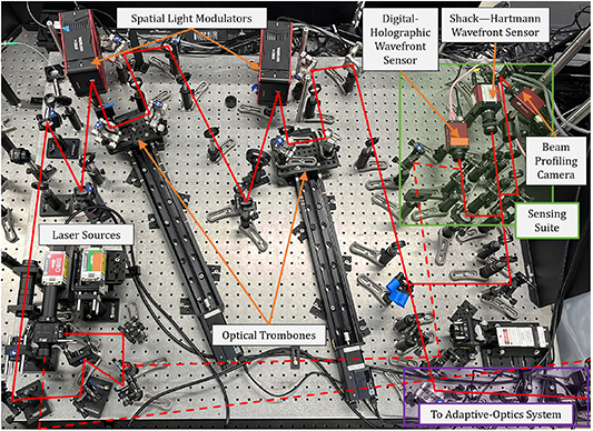
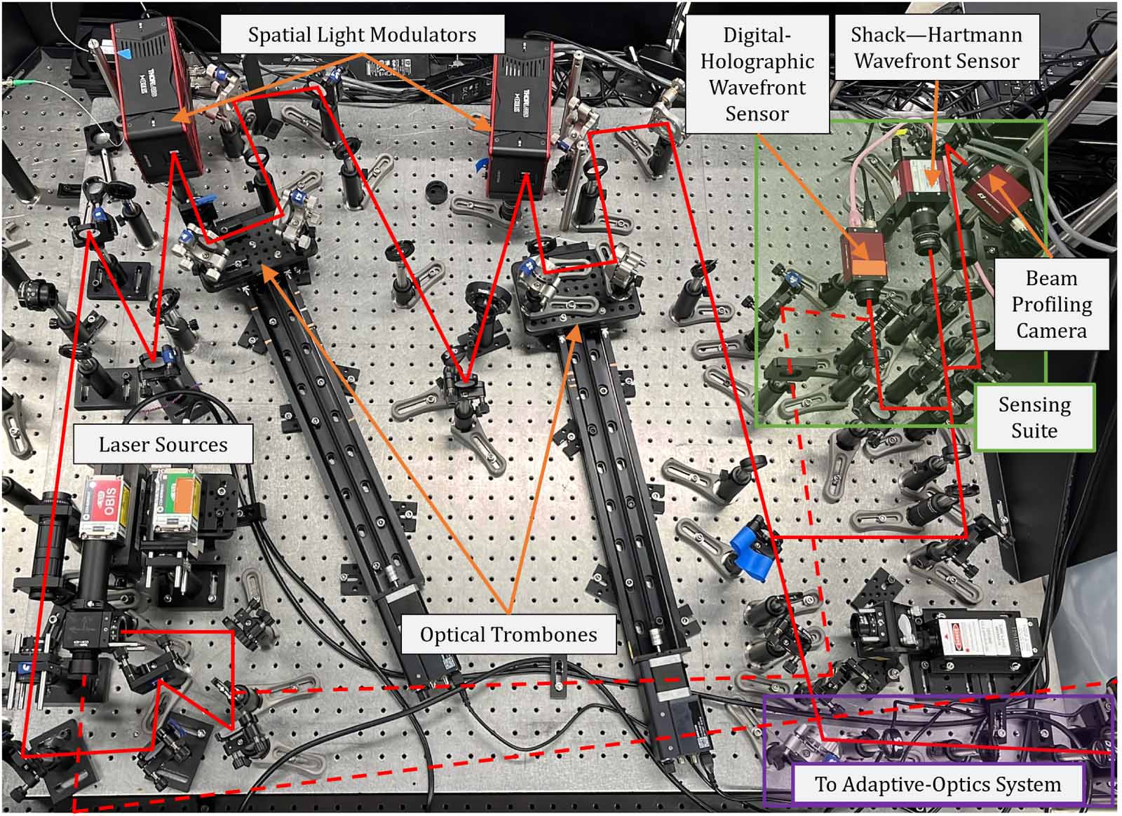
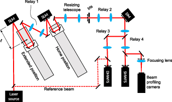
3.1.1. Optical setup.

We present an image of our ATS system in figure 1. The optical path begins at the bottom-left part of figure 1 where we have two laser sources installed; one with a central wavelength of 532 nm and another with a central wavelength of 633 nm. For the experiments presented in this paper, we only used the 633 nm laser source. For this source, we used a Coherent OBIS 633 single frequency laser that had a linewidth of $\lt\!0.3$ pm.

Figure 1. Schematic of the ATS.

Download figure:

Standard image High-resolution image

We first directed the laser beam through a beam splitter such that we had two different laser paths. We depict the first laser path with a solid-red line in figure 1 and this laser beam was transmitted through our ATS. We depict the second laser path with a dashed red line in figure 1 and this laser beam bypassed the ATS. Focusing on the laser beam transmitted through the ATS, we passed the laser beam through a half waveplate and then expanded the beam to be approximately 3.3 mm in diameter. We then directed the beam to our first spatial light modulator (SLM), located in the top-left part of figure 1. In this system, we used two Thorlabs Exulus HD1 SLMs to impose representative atmospheric-turbulence-induced phase aberrations onto the beam. This will be discussed in greater detail in the next section. These SLMs had a pixel pitch of 6.4 µm with a panel resolution of 1920 × 1080, corresponding to a panel size of 12.5 × 7.1 mm2 with a fill factor of $\gt\!93\%$ . The SLMs required 8 bit, gray-scale images and had a frame rate of 60 Hz. We positioned the SLMs at a slight angle relative to the incident beam such that we could spatially separate the reflected laser beam from the incoming laser beam without clipping, while also ensuring that the angle was within the specification defined by the SLM manufacturer. We directed the laser beam reflecting off the SLM to an optical trombone. An optical trombone is a pair of turning mirrors mounted on a linear actuator such that moving the linear actuator does not change the alignment of the laser beam. The optical trombone’s home position represents where the SLMs and system exit pupils are conjugate. We then replicated free-space propagation by extending the optical trombone away from its home position. With this system design, the phase screens that we apply to our SLMs dictate r0, while the combination of the phase screens that we apply to our SLMs as well as our optical-trombone positions dictate the $\mathcal$ conditions that we are replicating. We relayed the beam from one SLM to the next using a 4f relay comprised of two 300 mm lenses. The second SLM followed the same procedure as the first. Namely, we kept the SLM at a slight angle relative to the incident laser beam, directed the reflected laser beam to a second optical trombone, and then relayed the laser beam using two 300 mm lenses to the exit pupil of the system, located in the bottom-right portion of figure 1. We split the laser beam exiting the ATS into two different branches: one branch went to a diagnostic measurement suite located in the ATS (top-right part of figure 1) and the other branch was directed into our benchtop AO system (bottom-right part of figure 1). For the experiments described in this paper, we did not use the diagnostic measurement suite in the ATS and therefore, it will not be discussed.

3.1.2. Algorithm.

We used the SLMs to impose dynamic atmospheric-turbulence phase screens onto the laser beam reflecting off them. The phase screen generation followed the same procedure used in wave-optics simulations and outlined in [48–51]. Specifically, we generated the phase screens by filtering Gaussian white noise using the Kolmogorov power spectrum. For the experiments presented in this paper, we defined the phase screens to be 1.05 $\times$ 1.05 m2 in size and they consisted of 1024 $\times$ 1024 points. We varied $C_n^2$ depending on the atmospheric-turbulence condition that we were simulating, defined the total propagation distance to be L = 1 km, and defined the wavelength to be λ = 633 nm. We also selected the size of the beam that we sought to replicate to be 20 cm. This enabled us to spatially scale between the simulated atmospheric-turbulence phase screens and the laser beam reflecting off the SLMs. We allowed the phase screens to change dynamically by defining a ‘wind speed.’ Accordingly, each subsequent time step resulted in a translation of the atmospheric-turbulence-induced phase aberrations. For all cases, we defined the ‘wind speed’ to be 0.05 m s−1. We intentionally selected a slow ‘wind speed’ in order to generate low $f_\mathrm G$ conditions. As we will discuss in greater detail later on, we elected to do this such that we could focus on the quality of our spatial correction in our AO system, and not introduce any appreciable additional performance degradation associated with temporal bandwidth limitations. However, it is worth noting that while we chose slower ‘wind speeds’ for the experiments presented in this paper, our ATS can create ‘wind speed’ upwards of 10 m s−1—allowing us to create a diverse range of $f_\mathrm G$ conditions for future experiments that leverage our ATS.

After generating phase screens with the desired atmospheric-turbulence statistics, we resampled and cropped the phase screens to match the grid resolution and size of the SLMs. After which, we also introduced an additive tilt complex-phasor term onto each phase screen. We included the additive tilt in order to deflect the desired ‘signal’ beam away from the diffractive orders of the SLM. Lastly, we converted the originally continuous phase screen into a modulo-2π phase screen and scaled it to integer values between 0 and 255, as required by our SLMs. The procedure described above was carried out using an in-house-developed MATLAB code; however, we applied the phase screens to the SLMs using the software package provided by the SLM manufacturer.

3.2. Adaptive-optics (AO) system

In this section, we describe both the optical setup as well as the algorithm for the AO system.

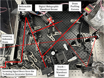
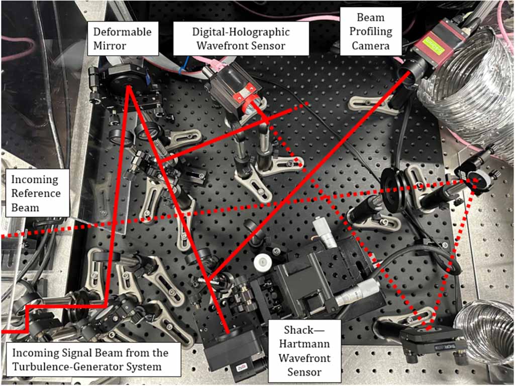
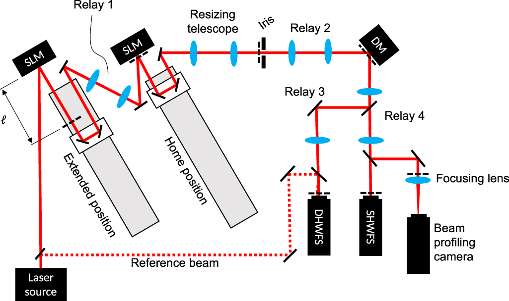
3.2.1. Optical setup.

After leaving the ATS, the laser beam entered our benchtop AO system. We present an image of our system in figure 2. Similar to figure 1, we will use figure 2 to assist with our discussion. Between the exit of the ATS and the entrance of the AO system (bottom-left part of figure 2), we magnified the laser beam such that the beam size matched the size of the active area on our DM. Subsequently, we 4f relayed the beam onto the DM. The DM we were using was a Boston Micromachines Corporation Multi-3.5 MEMS DM model. This DM consisted of a 12 $\times$ 12 array with the corner actuators missing, resulting in 140 total actuators. The actuators had a maximum physical stroke of 3.5 µm which resulted in a reflected wavefront stroke of 7 µm. The DM clear aperture diameter was 4.40 mm with an interactuator pitch of 400 µm. The actuator’s mechanical response was $\lt\!75$ µs (∼13.3 kHz). We minimized the angle between the incident and reflected laser beam from the DM in order to limit elongation of the beam on the DM’s active surface.

Figure 2. Schematic of the benchtop AO system with diagnostic instruments.

Download figure:

Standard image High-resolution image

After the DM, we demagnified and relayed the beam to a Thorlab’s WFS20-5 C Shack–Hartmann wavefront sensor (SHWFS). The SHWFS is depicted in the bottom-middle part of figure 2. The camera used for this SHWFS had a maximum resolution of 1440 × 1080 pixels with a pixel pitch of 5 µm; however, we only used the camera in the 1080 × 1080 pixel format, binned to a resolution of 540 × 540 pixels. The SHWFS lenslets had a pitch of 150 µm and focal lengths of 4.1 mm. We use the SHWFS to inform the AO correction on the DM. We will discuss the algorithm used to accomplish this in the next section.

Between the DM and the SHWFS, we also added two beam splitters. We used the first beam splitter to relay the laser beam from the DM to a digital-holographic wavefront sensor (DHWFS), located in the top-middle part of figure 2. DHWFSs are an interferometric-based wavefront sensing approach that enables access to the full complex-optical field of the laser beam. The DHWFS has been shown to be resilient to scintillation and branch points [52–54]. In our setup we used the off-axis pupil plane recording geometry, where the laser beam relayed from the DM was interfered with a collimated reference laser beam. This implementation of DHWFS has been heavily studied in the literature [53, 55–57]. Here, we used the portion of the 633 nm source that bypassed the ATS as the reference beam. Similar to figure 1, we depict the path of the reference beam using a dashed red line. We used two turning mirrors and another beam splitter to combine the laser beam from the DM and the reference beam onto the DHWFS. The camera we used for the DHWFS was an Allied Vision Alvium G5-130 camera. This camera had an InGaAs sensor with a resolution of 1296 × 1032 and a pixel pitch of 5 µm. For the experiments presented in this paper, we used the DHWFS measurements in order to compute turbulence statistics and to characterize our AO system performance. We collected all DHWFS measurements at a frame rate of 45 Hz for 10 s durations. We will discuss the DHWFS algorithm and data-reduction procedures in detail in section 3.3.1.

We used the second beam splitter between the DM and the SHWFS to direct the corrected beam towards a beam-profiling camera (located in the top-right part of figure 2). We focused the laser beam onto the beam-profiling camera using a 250 mm lens and we used these measurements to quantify the AO system performance. The beam-profiling camera was an Allied Vision Manta MG-040c. This camera had a CMOS sensor with a resolution of 728 × 544 and a pixel pitch of 6.9 µm. We collected all beam-profiling measurements at a frame rate of 60 Hz for 10 s durations. We will discuss the data reduction procedure for the beam-profiling measurements in section 3.3.2.

Recognizing the complexity of figures 1 and 2, to further assist the reader, we also present a simplified schematic of our ATS and AO systems in figure 3. Similar to figures 1 and 2, the solid red line represents our beam that transmitted through both our ATS and AO systems, while the dashed red line represents our reference beam that bypassed the ATS and AO systems and was used for our DHWFS measurements. The various dashed black lines in the figure denote the conjugate planes of the systems.

Figure 3. Simplified schematic of the ATS and AO systems. This example shows one SLM in its home position and the other in its extended position, adding an additional optical path length of $\ell$ .

Download figure:

Standard image High-resolution image 3.2.2. Algorithm.

As described above, we used a SHWFS to inform our AO correction. A SHWFS consists of an array of lenslets which focus incoming light onto a camera’s detector. The deviations of the resultant irradiance patterns away from their on-axis locations are proportional to the average phase tilts across each lenslet’s pupil. We approximate the local phase tilts in both the x and the y directions, θx and θy, by dividing the measured centroid deviations by the focal length of the SHWFS lenslets. For the experiments presented in this paper, we used an in-house-written algorithm to perform the SHWFS processing.

In order to operate the AO system, we first needed to perform a calibration procedure. To do so, we removed atmospheric-turbulence phase screens from the SLMs and we set our DM to its ‘flat’ position. We then sequentially ‘poked’ each DM actuator with a known amplitude and measured the resultant response on the SHWFS. This enabled us to relate the DM actuator ‘pokes’ to the measured SHWFS response as $\boldsymbol$ , where p was the vector of known ‘poke’ amplitudes for each DM actuator, and $\boldsymbol = \left[\begin \theta_x \\ \theta_y \end\right]$ was a matrix containing the x and y tilts measured by the SHWFS. Solving for A resulted in a matrix size that was twice the number of SHWFS centroid measurements by the number of DM actuators. Inverting this matrix with the Moore–Penrose pseudo-inverse gave $\boldsymbol^$ , which we refer to as the ‘reconstructor’ matrix.

Once this calibration was complete, we could calculate the DM actuator amplitudes needed to compensate for an unknown disturbance from a set of θx and θy measurements. Specifically, we accomplished this by solving the linear equation $\boldsymbol = \boldsymbol^\boldsymbol$ . From here, we used p in order to generate our DM command. To accomplish this, we first calculated our correction estimate as $\boldsymbol_i = K\boldsymbol_i+c\boldsymbol_$ , where i indicates the time step, K is a gain, and c is a leaky integrator coefficient. In writing, we calculated our new correction estimate by multiplying our calculated DM actuator amplitudes by a gain plus the previous correction estimate multiplied by a leaky integrator coefficient. Our DM command, $\boldsymbol$ was then $\boldsymbol} = -\boldsymbol_i+\boldsymbol$ , where f were DM actuator amplitudes corresponding to ‘flat’ data provided by the vendor.

To summarize our AO algorithm, we collected a SHWFS frame, processed the SHWFS data to obtain θ, subsequently calculated p, and then used p to arrive at our DM command $\boldsymbol$ . We conducted this logic in closed-loop fashion. For the experiments discussed in this paper, we defined K = 0.4, c = 0.99, and the loop rate of the AO compensation was ≈ 90 Hz. Note, we selected the parameters K = 0.4 and c = 0.99 based on prior experimental testing which suggested that these parameters created a stable, yet responsive control loop.

3.3. Data collection and processing

In this section, we discuss the data collection and processing procedures associated with both the DHWFS and the beam-profiling camera.

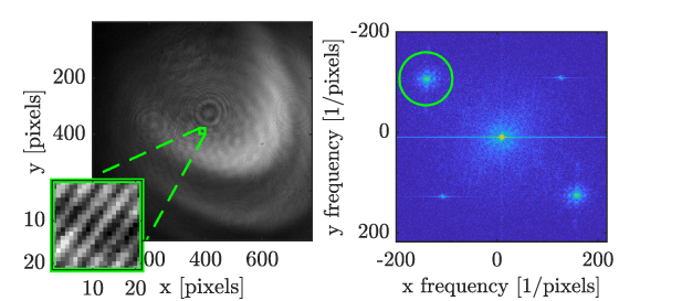
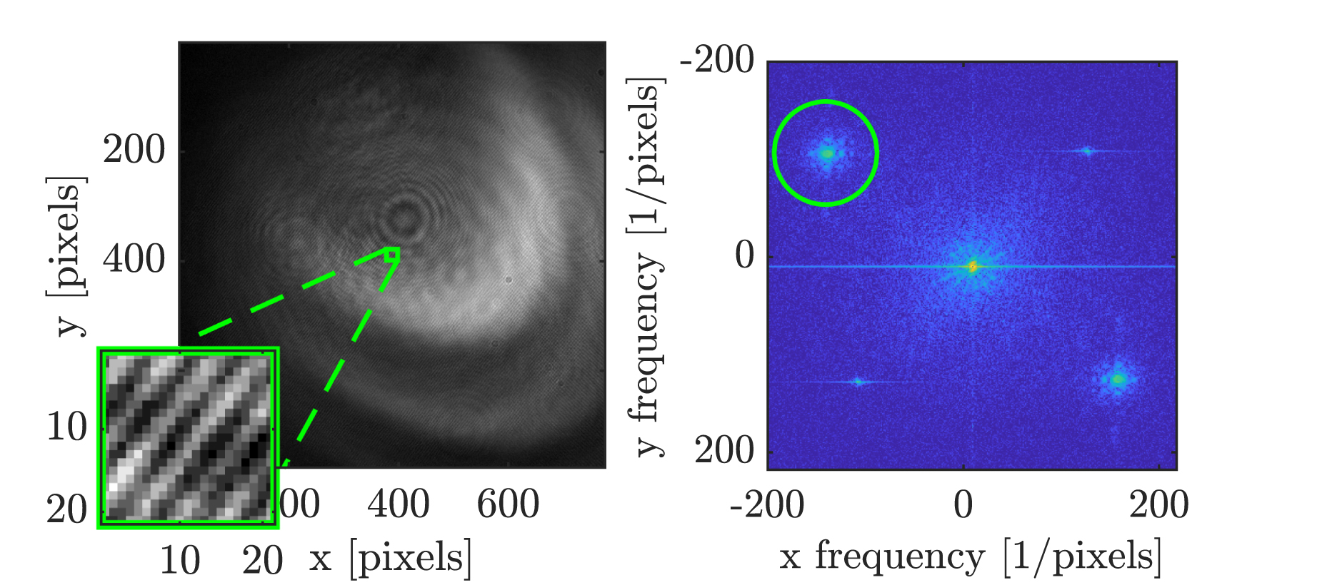
3.3.1. DHWFS.

As discussed above, the DHWFS is a wavefront sensing technique that allowed us to gain access to the complex-optical field of the laser beam. Our setup used an off-axis pupil plane recording geometry where we interfered the laser beam relayed from the DM with a tilted planar reference beam onto a camera sensor, which created an interference pattern or hologram. We present an example hologram in the left plot of figure 4. We also present a zoomed-in view of the interference pattern in the bottom-left part of the image. From here, we performed a two-dimensional fast Fourier transform on the hologram, which allowed us to isolate the signal-reference crossterm in the Fourier plane. By adding tilt to the reference beam, we could separate the signal-reference crossterm from the autocorrelative noise in the center of the Fourier plane. From here, we could then apply a low-pass filter to isolate this term, which is shown with a green circle in the right plot of figure 4. Subsequently, we shift the crossterm to the origin (i.e. recenter it) in order to remove tilt. The diameter of the low-pass filter was selected to balance minimizing noise, while also still capturing relevant small-scale turbulence distortions. An inverse Fourier transform then returns the desired complex-optical field. References [57–59] describe this process in greater detail.

Figure 4. Processing steps of digital holography. The left plot shows the hologram measured on camera. The right plot shows the magnitude of the two-dimensional fast Fourier transform of the hologram.

Download figure:

Standard image High-resolution image

Using the complex-optical fields obtained from the DHWFS measurements, we could then access both the amplitude and wrapped phase functions. Furthermore, we could decompose the wrapped phase function of the complex-optical field into two components: the continuous, or least-squares component of phase, as well as the rotational component of phase, referred to by many as the ‘hidden’ phase. To calculate the least-squares component of phase, we first used the wrapped phase field to calculate phase gradients in the x and y directions. Subsequently, we used the phase gradients in a least-squares reconstruction algorithm. In order to obtain the hidden phase field, we multiplied a complex phasor containing the wrapped phase by the complex conjugate of a phasor containing the least-squares component of phase. As we show in section 4, we used both the least-squares and hidden phase fields measured using the DHWFS to help quantify AO system performance.

Prior to collecting data with the DHWFS, it is customary to collect a set of baseline DHWFS measurements. To collect these baseline DHWFS measurements, we removed atmospheric-turbulence phase screens from the SLMs and we set our DM to its ‘flat’ position. We process these baseline DHWFS measurements using the procedure described above in order to obtain a measurement of the aberrations local to the ATS and AO system. We then divided the complex-optical fields of our data collections by the complex-optical field processed from these baseline measurements to, in essence, remove the effect of aberrations local to our system.

3.3.2. Beam-profiling camera.

As discussed in section 3.2.1, after relaying the laser beam from the DM, we focused the laser beam onto a beam-profiling camera. We used the measurements from this camera in order to quantify AO system performance. Specifically, we collected irradiance images of the focused laser beam in order to calculate normalized power-in-the-bucket, nPIB. Before applying atmospheric-turbulence phase screens to the SLMs and while the DM was set to its ‘flat’ position, we collected beam-profiling data that we used as a reference data set.

In order to measure nPIB, we first calculated the centroid of the focused laser beam on a frame-by-frame basis. From here, we summed the irradiance values within a ‘bucket’ surrounding the calculated centroid. We selected the diameter of the ‘bucket’ to be the $1/e^2$ diameter calculated from the reference beam-profiling results. For the experiments presented in this paper, we found this diameter to be 0.11 mm (which is approximately twice our diffraction-limited spot size). The power-in-the-bucket measured for each data point was normalized by the power-in-the-bucket for the reference case in order to obtain nPIB.

Before moving on, it is worth noting that the frame-by-frame manner in which we calculated nPIB made our results serve as tilt-removed, or jitter-removed AO results. As discussed in section 1, in this paper, we focused on the AO functionality of the beam-control system. Since our system did not have tracking functionality, we had uncompensated tilt on the laser beam resulting in tilt in our DHWFS measurements as well as beam jitter in our beam-profiling measurements. For this reason, we removed all tilt from the phase fields reconstructed using the DHWFS measurements and we calculated nPIB with respect to the measured centroid locations and not the on-axis location—allowing us to explore AO performance degradation due to beam spreading as opposed to beam jitter.

In this section, we discuss the experimental trade space that we explored (section 4.1). We also present and discuss the results of this trade space. The results are broken into two parts: results that discuss optical-turbulence statistics (section 4.2) and results that discuss AO performance (section 4.3).

4.1. Experiment trade space

In addition to our baseline data collections, we used our ATS to generate 13 different optical-turbulence conditions corresponding to $D/r_0$ values ranging from 0.50 to 12. To accomplish this, we generated dynamic atmospheric-turbulence phase screens using the approach described in section 3.1.2 and we applied these dynamic phase screens to one of our two SLMs in the ATS. For each of the turbulence conditions that we explored, we generated 10 different Monte–Carlo instances such that we could ensemble average our results. Note, for a similar type of analysis conducted in wave-optics simulations, one would likely want to conduct many more than 10 independent realizations. However, given the time required to collect these experimental measurements, 10 independent realizations per turbulence condition is what was feasible and as we will show, yielded excellent results. We present a complete parameterization of the optical-turbulence trade space that we explored in table 1.