6.1 Generalized Quantum Non-demolition

Let us now consider a case where all the operators are block-diagonal in the same basis. This represents a generalization of the quantum non-demolition (QND) condition, which will be later derived as a special case.

Consider an Hilbert space

$$\begin \mathcal =\bigoplus _^K \mathcal _k. \end$$

This decomposition of the Hilbert space induces a natural block-decomposition of the set of operators \(\mathfrak (\mathcal )\). In the following we consider operators that are block-diagonal in the block-decomposition induced by the decomposition of \(\mathcal \).

As announced, an important model which fits this situation is the so-called quantum non-demolition measurement model. This case is given by one-dimensional component \(}_k=}\vert e_k\rangle \), where \(\\) is an orthonormal basis for \(\mathcal \). This basis is called a pointer basis and the involved operators are diagonal in this basis. When studying the long-time behavior of the monitored system under non-demolition measurements, the quantities \((\textrm(\vert e_l\rangle \langle e_l\vert \rho _t)), l=1,\ldots ,K\) play a crucial role. It is then natural to consider our reduction model in this situation. In particular we study the general case where block diagonal is of any dimension (not only one)

6.1.1 Generalized QND

Consider a Hamiltonian, noise operators and measurement operators that are block-diagonal in the basis provided by this decomposition of the Hilbert space \(\mathcal \), i.e.,

$$\begin H= \bigoplus _^K H_k, \qquad L_j= \bigoplus _^K L_, \qquad D_j = \bigoplus _^K D_, \quad \text \quad C_j = \bigoplus _^K C_ \end$$

with \(H_k,L_,D_,C_\in \mathfrak (\mathcal _k)\). We further assume to be interested in reproducing the expectation value observables \(O_j\) that are also block-diagonal:

$$\begin O_j = \bigoplus _^K O_ \end$$

where \(O_\in \mathfrak (\mathcal _k)\). As an example one can consider to be interested in reproducing the probability of the state being in each of the subspaces \(\mathcal _j,\) which implies the observables of interest are the orthogonal projectors onto each \(\mathcal _j\). In order to satisfy both Assumptions 1 and 2, we need to include \(\mathbbm \), \(D_j+D_j^*\) and \(C_j^* C_j\) to the set of observables of interest. One can easily verify that these operators are block-diagonal as well.

For generic choices of the diagonal blocks, the space orthogonal to the non-observable space \(\mathscr ^\perp \) generates the entire block-diagonal algebra

$$\begin \mathscr = \bigoplus _^K \mathfrak (\mathcal _k). \end$$

Note that, it is possible, for specific choices of the diagonal blocks, that the non-observable space is such that \(\mathscr ^\perp \subseteq \textrm(\mathscr ^\perp )\subsetneq \mathscr \) or, in other words, a smaller reduction could exist. An example of this is shown in the next subsection. Furthermore, for any choice of the diagonal blocks of \(L_j,D_j,C_j\) and \(O_j\), the algebra \(\mathscr \) contains \(\textrm\\), is \(\mathcal ^*\)-, \(\mathcal _^*\)- \(\mathcal ^*_\)-invariant (trivially since sums and products of block-diagonal matrices remain block-diagonal); hence, in general, we have \(\mathscr ^\perp \subseteq \textrm(\mathscr ^\perp ) \subseteq \mathscr \). This shows that, albeit in certain cases the reduction of the filter onto \(\mathscr \) could be non-minimal, it is always possible to reduce the filter onto \(\mathscr \).

In such a case the reduction and injection superoperators result to be

$$\begin \mathcal _\mathscr (X)&\equiv \bigoplus _^K V_k^* X V_k = \bigoplus _^K X_k = \check,\\ \mathcal _\mathscr (\check)&\equiv \check \end$$

where \(V_k = \left| k \right\rangle \otimes \mathbbm __k}\) are the isometries \(V_k:\mathcal _k\rightarrow \mathcal \).

The reduced un-normalized state

$$\begin \check_t = \mathcal _\mathscr (\tau _t) = \bigoplus _^K \check_ \end$$

then evolves according to the linear stochastic differential equation

$$\begin&d\check_ = \check}_(\check_)dt + \sum _^\mathcal __}(\check_) dY_t^j \\&\quad +\sum _^q \left[ \mathcal __}-\mathcal _}}\right] (\check_) (dN_t^j-dt) \qquad \forall k=1,\dots ,M \end$$

where

$$\begin & \check}_(\check) = -i[H_k,\check] + \sum _^\mathcal _}(\check) \\ & \quad + \sum _^\mathcal _}(\check) + \sum _^\mathcal _}(\check).\end$$

With this, one can observe that each block \(\check_\) of the un-normalized state \(\check_\) evolves independently of all the others. This is not the case when considering the normalized state

$$\begin \check_t = \frac_t}(\check_t)}= \mathcal _\mathscr (\rho _t) = \bigoplus _^K \check_ \end$$

where each block evolves trough the SME

$$\begin&d\check_ = \check}_k(\check_) dt + \sum _^ \left[ \mathcal _}(\check_) - \check_\sum _^K\textrm[\mathcal _}(\check_)] \right] \\&\quad \left( dY_t^j - \sum _^K\textrm[\mathcal _}(\check_)] dt\right) \\ &+ \sum _^\left[ \frac_}(\check_)}^K\textrm[\mathcal _}(\check_)]}-\check_\right] \left( dN_t^j-\sum _^K\textrm[\mathcal _}(\check_)]dt\right) , \end$$

which clearly depends on all the blocks (see also the discussion in [6]).

The expectation values of interest is then obtained as

$$\begin \textrm[O_j \rho _t] = \sum _^K\textrm[O_\check_] = \frac^K\textrm[O_\check_]}^K\textrm[\check_]}. \end$$

Note that the fact that each block of the reduced un-normalized state \(\check_t\) evolves independently of the others might provide a computational simulation advantage. In fact, to simulate the expectation values of interest, one can simulate each block \(\check_\) independently, either in parallel or in series depending on the available resources, and then sum the results to obtain the desired expectation values. Notice that the potential for independent block simulation for the average semigroup dynamics was also found in [35] in presence of strong symmetries, albeit in that case the evolution is already linear and can be simulated directly in block form.

6.1.2 Quantum Non-demolition Continuous Measurement

As a special case of the example we just presented, we can focus on quantum non-demolition measurements in continuous time. Consider an Hamiltonian and noise operators that are block-diagonal in the basis provided by the decomposition of the Hilbert space \(\mathcal \), i.e.,

$$\begin H= \bigoplus _^K H_k, \qquad \text \qquad L_j= \bigoplus _^K L_ \end$$

with \(H_k,L_\in \mathfrak (\mathcal _k)\). Furthermore, let us consider measurement operators that, in each diagonal block, are proportional to the identity operator acting on the relative subspace \(\mathcal _k\), i.e.,

$$\begin \qquad D_j = \bigoplus _^K d_\mathbbm __}, \qquad \text \qquad C_j = \bigoplus _^K c_ \mathbbm __k} \end$$

with \(d_,c_\in \mathbb \). Assume then that we are interested in reproducing the probability of the state being in each of the subspaces \(\mathcal _j\), i.e., we consider the observables of interest \(O_j\) to be the orthogonal projectors onto \(\mathcal _j\):

$$\begin O_j = \bigoplus _^K \mathbbm __k}\delta _\qquad \forall j=1,\dots ,K, \end$$

where \(\delta _\) denotes the Kronecker delta. With this, one can verify that both Assumptions 1 and 2 are satisfied, and we can thus proceed with our proposed procedure. Note that the typical QND setting [19, 48] can be seen as a special case where \(\dim (\mathcal _k)=1\) for all k or where \(H, L_j\) are also diagonal in the standard basis.

As a first step, we shall compute the operator subspace \(\mathscr ^\perp \). From the properties of the non-observable subspace presented in Proposition 1 we know that \(\textrm\_^K\subseteq \mathscr ^\perp \). We also know that \(\mathscr ^\perp \) is also \(\mathcal ^*\)- \(\mathcal _^*\)- and \(\mathcal _^*\)-invariant. One can then observe that \(\textrm\_^K\) is \(\mathcal _^*\)- and \(\mathcal _^*\)-invariant since

$$\begin \mathcal _^*(O_h)&= D_j O_h + O_h D_j^* = \bigoplus _^K 2d_\delta _\mathbbm __k},\\ \mathcal _^*(O_h)&= C_j^* O_h C_j = \bigoplus _^K c_^2\delta _\mathbbm __k}. \end$$

Verifying that \(\textrm\_^K\) is also \(\mathcal ^*\)-invariant is also straightforward. One can in fact verify that \(\textrm\_^K\) is contained in \(\ker \mathcal ^*\) by computing:

$$\begin H,O_h]&= HO_h - O_hH = \bigoplus _^K [H_k, \mathbbm __k}]\delta _ = 0\\ \mathcal _^*(O_h)&= L_j^* O_h L_j -\frac\ = \bigoplus _^K (L_^* \mathbbm __k} L_ \\&\quad - \frac \^* L_, \mathbbm __k}\} )\delta _=0, \end$$

and \(\mathcal _^*(O_h) = 0\) and \(\mathcal _^*(O_h)=0\).

Then, since \(\textrm\_^K\) is \(\mathcal ^*\)-, \(\mathcal _^*\)-, and \(\mathcal _^*\)-invariant and is trivially the smallest operators subspace that contains itself we find

$$\begin \mathscr ^\perp = \textrm\_^K. \end$$

To proceed with the reduction procedure, one should then find the algebra \(\textrm(\mathscr ^\perp )\) generated by the subspace \(\mathscr ^\perp \). One can, however, notice that \(\mathscr ^\perp \) is already an abelian algebra of dimension M; hence,

$$\begin \mathscr = \textrm\_^K = \bigoplus _^K \mathbb \mathbbm __k} \end$$

where we also expressed its Wedderburn decomposition. This allows us to write the reduction and injection superoperators that factor the conditional expectation:

$$\begin \mathcal _\mathscr (X)&\equiv \bigoplus _^K \textrm[ V_k^* X V_k] = \bigoplus _^K x_k = \check \quad \in \mathbb ^K \\ \mathcal _\mathscr (\check)&\equiv \bigoplus _^K x_k \mathbbm __k}, \end$$

where \(V_k = \left| k \right\rangle \otimes \mathbbm __k}\) are the isometries \(V_k:\mathcal _k\rightarrow \mathcal \).

We finally have all the elements to compute the reduced model. First of all, one can notice that the action of the Lindblad generator on the algebra is null, i.e., \(\mathcal \circ \mathcal = 0\); hence, there is no need in computing the reduced Hamiltonian and noise operators since \(\check}=0\).

For the measurement operators, the reduction process is quite simple. First of all, we can notice that, by assumption, both \(D_j\) and \(C_j\) are all block-diagonal. This implies that the reduced operators will also result (block-)diagonal (in the terminology used in “Appendix A” we only have \(e=0\)). We then need to construct an orthonormal operator basis for the spaces that get factored out and express the original operators in that basis. Let us consider a set of operator basis \(\\) for the spaces \(\mathfrak (\mathcal _k)\) such that \(E_0^k=\mathbbm __k}/\dim (\mathcal _k)^\frac\) for all k. Then the original measurement operators can be written as

$$\begin \qquad D_j = \bigoplus _^K d_\dim (\mathcal _k)^\fracE_0^k, \qquad C_j = \bigoplus _^K c_\dim (\mathcal _k)^\fracE_0^k. \end$$

Using then Proposition 2, we can then directly compute the reduced measurement operators:

$$\begin D_j \,\rightarrow \, \check_j = \bigoplus _^K d_,\qquad C_j \,\rightarrow \, \check_j = \bigoplus _^K c_ . \end$$

The reduced state

$$\begin \check_t = \mathcal _\mathscr (\rho _t) = \bigoplus _^K p_ \end$$

with \(p_\in [0,1]\) and \(\sum _^K p_ =1\), \(\forall t\ge 0\) then evolves according to the SME

$$\begin d\check_t & = \sum _^p (\mathcal __j}(\check_) - \textrm[\mathcal __j}(\check_)]\check_) dW_t^j \\ & \quad + \sum _^q\left( \frac__j}(\check_)}[\mathcal __j}(\check_)]} - \check_ \right) (dN_t^j-\textrm[\mathcal __j}(\check_)]). \end$$

Because the reduced state \(\check_t\) is diagonal, one can also represent the same evolution explicitly expressing each diagonal element, obtaining

$$\begin dp_ & = \sum _^p \left( 2d_p_- p_ \sum _^K 2d_p_ \right) dW_t^j \\ & \quad + \sum _^q \left( \frac^2 p_}^K c_^2 p_}-p_\right) \left( dN_t^j - \sum _^K c_^2 p_\right) \end$$

rediscovering the form found in [19]. The probability of the state being in a subspace \(\mathcal _j\) can then be computed as

$$\begin \textrm[O_j \rho _t] = \textrm[\check_j \check_t] = p_ \end$$

where \(\check_j = \left| j \big \rangle \big \langle j \right| \).

6.2 Measured Spin Chains

We consider here a model consisting of a spin chain undergoing both homodyne- and counting-type measurement. Specifically, we here consider a model composed by N qubits, i.e., \(\mathcal = \otimes _^N \mathcal _j\) with \(\mathcal _j \simeq \mathbb ^2\). Let then \(\sigma _q\) with \(q\in \\) denote the usual Pauli matrices with \(\sigma _0\equiv \mathbbm _2\) and

$$\begin \sigma _q^ \equiv \mathbbm _} \otimes \sigma _q \otimes \mathbbm _} \end$$

the operators in \(\mathfrak (\mathcal ) = \mathbb ^\times 2^N}\) that act non-trivially only on the j-th qubit. Similarly, we denote by \(\sigma _\pm ^\equiv \frac\left( \sigma _x^\pm i\sigma _y^\right) \) local raising and lowering operators. Whenever there is no confusion on the space onto which \(\sigma _q^\) acts, we drop the dependence on N using the symbol \(\sigma _q^\).

6.2.1 Model Description

We assume that the spins in the chain interact trough an inhomogeneous Ising Hamiltonian with transverse field, which reads

$$\begin H = \sum _^ \delta _j \sigma _x^\sigma _x^ + \sum _^N \mu _j \sigma _z^, \end$$

(27)

with \(\delta _j,\mu _j\in \mathbb \). Furthermore, the entire system undergoes continuous-time local measurement described by the operator

$$\begin D_j \equiv \gamma _j \sigma _z^, \qquad \forall j = 1,\dots , N \end$$

as well as counting-type measurements described by the operators

$$\begin C_j \equiv \alpha _j \sigma _-^, \qquad \forall j=1,\dots ,N. \end$$

These measurement operators can be considered either as physical description of measurement processes such as photon emission (or absorptionFootnote 1), or as unravelings of Lindblad generators [56, 64]. While the simultaneous continuous- and counting-type measurement considered in this example might not be physically realistic, handling both of them presents no mathematical challenge. More importantly, as we shall see, this model allows us to study the effects of off-diagonal blocks that can be present only in counting-type measurement operators. For these reasons, we consider and reduce the model with both processes. Removing either counting-type or continuous type measurement is possible by simply setting the parameters \(\alpha _j\) or \(\gamma _j\) to zero.

One could then be interested, for example, in reproducing the probability distribution in the standard basis, i.e., the considered observables of interest are

$$\begin O_k = \left| k \big \rangle \big \langle k \right| , \qquad \forall k = 1,\dots ,2^. \end$$

With this, one can verify that, \(D_j+D_j^*\in \textrm\_^\), since \(D_j\) are diagonal in the basis given by \(\left| k \right\rangle \), as well as \(C_j^* C_j\in \textrm\_^\) since

$$\begin }^*\sigma _^ = \sigma _^\sigma _+^ = \mathbbm _} \otimes \left| 1 \big \rangle \big \langle 1 \right| \otimes \mathbbm _},\\ }^*\sigma _^ = \sigma _^\sigma _-^ = \mathbbm _} \otimes \left| 0 \big \rangle \big \langle 0 \right| \otimes \mathbbm _}; \end$$

hence, both assumptions 1 and 2 are satisfied. Note that, since \(D_j\in \textrm\_^\), the reduced model is also able to reproduce the expectation value of the local magnetization \(\left\langle \sigma _z^ \right\rangle \) as well as the probability distribution \(\left\langle O_k \right\rangle \).

6.2.2 Numerical Reduction for \(N=2,3\)

To perform the proposed model reduction procedure, one can then compute the superoperator algebra \(\mathscr \), the space orthogonal to the non-observable space \(\mathscr ^\perp \) defined in Proposition 1, compute the algebra \(\textrm(\mathscr ^\perp )\), the conditional expectation and its two factors \(\mathbb _}\), and then compute the reduced model as described in “Appendix A”.

Note that, in principle, these tasks can be performed on a (classical) computer by obtaining numerically the required spaces, algebras and operators. This, however, can be computationally demanding (the computation of \(\mathscr \) in particular) and depends on the size and the complexity of the dynamics for the system at hand. For this toy model, for example, we were able to compute numerically the spaces of interest, \(\mathscr ^\perp \) and \(\textrm(\mathscr ^\perp )\) as well as the reduced Hamiltonian and noise operators only for \(N=2,3\).

Specifically, for \(N=2,3\) we numerically verified that

$$\begin \textrm(\mathscr ^\perp ) \!=\! \textrm\left( \\}_^N\cup \\sigma _x^\}_^\right) \!\simeq \! \mathbb ^ \times 2^} \oplus \mathbb ^ \times 2^}.\nonumber \\ \end$$

(28)

While the computational complexity of the numerical methods might constrain us to reduce numerically only systems of small sizes, the intuition we can develop for systems of small sizes, as well as the theoretical results we developed in this work, allows us to extend some of the results theoretically to larger systems. This is in fact the approach undertaken in the next subsection, where we compute a sub-optimal reduced model that can provably be defined for any system size N and is inspired by the numerical computations we just described.

6.2.3 Sub-optimal Reduction for Any N

Although it may be difficult to analytically compute \(\mathscr ^\perp \), we can take inspiration from the numerically computed \(*\)-algebra given in (28) and define the algebra

$$\begin \mathscr \equiv \textrm\left( \\}_^N\cup \\sigma _x^\}_^\right) \end$$

with \(N\ge 2\). We might then wonder if, at least, such an algebra contains \(\mathscr ^\perp ,\) which would be a sufficient condition for reduction. The following Lemma answers this question.

Lemma 2

For the measured spin chain example described above and for \(\mathscr \), we have:

1.

\(\textrm\_^\subset \mathscr \);

2.

\(\mathscr \) is \(\mathcal ^*\)-, \(\mathcal _^*\)- and \(\mathcal _^*\)-invariant for all \(j=1,\dots ,N\);

3.

\(\textrm(\mathscr ^\perp )\subseteq \mathscr \).

Proof

Let us start by defining \(\mathscr _0\equiv \textrm\\}_^N = \textrm\_^}\) where \(\_^\) forms the standard basis for \(\mathcal \) and \(O_j\) are the observables of interest. By definition of \(\mathscr \) we have that \(\mathscr _0\subset \mathscr \); hence, \(\textrm\_^N\subset \mathscr \).

To prove the second claim, we can observe that \(H\in \mathscr \) hence, \(\mathscr \) is invariant under the action of \([H,\cdot ]\), i.e., \([H,X]\in \mathscr \) for all \(X\in \mathscr \). Similarly, since \(D_j\in \mathscr \), we have that \(\mathscr \) is also \(\mathcal _^*\)- and \(\mathcal _^*\)-invariant. It thus remains to prove that \(\mathscr \) is \(\mathcal _^*\)- and \(\mathcal _^*\)-invariant. Let us first observe that for any operator \(X\in \mathfrak (\mathcal )\), we have \(Q C_j^* X C_j Q^* = C_j^* Q X Q^* C_j\) where \(Q\equiv \prod _^N \sigma _z^\). Direct calculations lead to

$$\begin Q C_j^* X C_j Q^*&= F \underbrace \sigma _+^}_} X \underbrace \sigma _z^}_} F = F \sigma _+^ X \sigma _-^ F\\ C_j^* Q X Q^* C_j&= \underbrace \sigma _z^}_} F X F \underbrace \sigma _-^}_} = F \sigma _+^ X \sigma _-^ F \end$$

where we defined \(F\equiv \prod _ \sigma _z^\) for convenience. Then, since the superoperators \(\mathcal _^*\) and \(\mathcal (X)\equiv Q X Q^*\) commute, they share the same eigen-decomposition and, more importantly, every eigenspace of \(\mathcal \) is \(\mathcal _^*\)-invariant, see, e.g., [35, Sec. V.B] or [26]. In particular, we shell note that the 1-eigenspace of \(\mathcal \) coincides with \(\' = \mathscr \) and is \(\mathcal _^*\)-invariant. This proves that \(\mathscr \) is \(\mathcal _^*\)-invariant. The proof of the fact that \(\mathscr \) is also \(\mathcal _^*\)-invariant follows from this fact and from the fact that \(C_j^* C_j\in \mathscr \).

From the first and second claim, we have that \(\mathscr ^\perp \subseteq \mathscr \) by Proposition 1, i.e., the fact that \(\mathscr ^\perp \) is the smallest operator space that contains \(\textrm\\) and that is \(\mathcal ^*\)-, \(\mathcal _^*\)- and \(\mathcal _^*\)-invariant for all j. Then, by definition of \(\textrm\) we have that \(\textrm(\mathscr ^\perp )\) is the smallest operator \(*\)-algebra that contains \(\mathscr ^\perp \); hence, \(\mathscr ^\perp \subseteq \textrm(\mathscr ^\perp )\subseteq \mathscr \). \(\square \)

This lemma allows us to conclude that we can reduce the spin chain quantum filter onto the algebra \(\mathscr \), regardless of the number of spins N. Note that we here only proved that \(\textrm(\mathscr ^\perp ) \subseteq \mathscr \) hence, in principle, there could be smaller model than the one we compute next. We next show how to unitarily obtain the Wedderburn decomposition of the operators in the algebra \(\mathscr ,\) which we need in order to find the reduced model.

Lemma 3

Let us define the permutation matrix

$$P \equiv \mathbbm _4 + \sigma _x\otimes \mathbbm _2 + \mathbbm _2\otimes \sigma _z -\sigma _x\otimes \sigma _z = \begin 1& 0& 0& 0\\ 0& 0& 0& 1\\ 0& 0& 1& 0\\ 0& 1& 0& 0 \end \in \mathbb ^$$

and define, for any \(N\ge 1\), the unitary operator

$$U_N = \mathbbm _2 & \text N=1\\ (P\otimes \mathbbm _})(\mathbbm _2\otimes U_) & \text N\ge 2 \end\right. }.$$

Then for all N:

1.

$$U_N \sigma _z^ U_N^* = \sigma _z^\sigma _z^& \text j<N\\ \sigma _z^& \text j=N \end\right. };$$

2.

\(U_N \sigma _x^\sigma _x^ U_N^* = \sigma _x^\);

3.

\(U_N \mathscr U_N^* = \mathfrak (\mathbb ^}) \bigoplus \mathfrak (\mathbb ^})\);

4.

$$U_N \sigma _-^ U_N^* = \frac\left[ \sigma _x^\sigma _x^\dots \sigma _x^\sigma _x^ -i \sigma _x^\sigma _x^\dots \sigma _x^\sigma _y^ \sigma _z^ \right] & \text j < N\\ \sigma _x^\sigma _x^\dots \sigma _x^\sigma _-^& \text j=N \end\right. }. $$

Proof

Note that the fact that \(U_N\) is unitary can be easily proven by induction. The first claim of this lemma is also proven by induction. We start by proving the case \(N=2\). Simple calculations show that

$$\begin U_2\sigma _z^ U_2^*&= P (\sigma _z\otimes \mathbbm _2) P^* = \sigma _z\otimes \sigma _z\\ U_2\sigma _z^ U_2^*&= P (\mathbbm _2\otimes \sigma _z) P^* = \mathbbm _2\otimes \sigma _z. \end$$

Now assume that \(U_\sigma _z^U_^* = \sigma _z^\sigma _z^\) for \(j<N-1\) and \(U_\sigma _z^U_^* = \sigma _z^\). Then,

$$\begin&U_N\sigma _z^ U_N^* \\&\quad = (P\otimes \mathbbm _})(\mathbbm _2\otimes U_) (\sigma _z\otimes \mathbbm _}) (\mathbbm _2\otimes U_^*) (P^*\otimes \mathbbm _})\\&\quad = P(\sigma _z\otimes \mathbbm _2)P^* \otimes \mathbbm _} = \sigma _z\otimes \sigma _z\otimes \mathbbm _} = \sigma _z^\sigma _z^, \end$$

and, for \(j\ge 2\)

$$\begin&U_N\sigma _z^ U_N^* \\&\quad = (P\otimes \mathbbm _})(\mathbbm _2\otimes U_) (\mathbbm _2\otimes \sigma _z^) (\mathbbm _2\otimes U_^*) (P^*\otimes \mathbbm _})\\&\quad = (P\otimes \mathbbm _})(\mathbbm _2\otimes \sigma _z^\sigma _z^) (P^*\otimes \mathbbm _}) \\&\quad = (\mathbbm _2\otimes \sigma _z^\sigma _z^) = \sigma _z^\sigma _z^ \end$$

concluding the proof of the third point.

The next point is also proven by induction. We then prove the base case \(N=2\). Simple calculations show that \(U_2\sigma _x^\sigma _x^ U_2^* = P (\sigma _x\otimes \sigma _x) P^* = \mathbbm _2\otimes \sigma _x\) concluding the base case. Similar calculations show that \(P(\sigma _x\otimes \mathbbm _2)P^* = \sigma _x\otimes \mathbbm _2 \) and \(P(\mathbbm _2\otimes \sigma _x)P^* = \sigma _x\otimes \sigma _x \) which are useful in what comes next. We then assume that \(U_ \sigma _x^\sigma _x^ U_ = \sigma _x^\) and consider

$$\begin U_N \sigma _x^\sigma _x^U_N^*&= (P\otimes \mathbbm _})(\mathbbm _2\otimes U_) (\sigma _x\otimes \sigma _x^)\\&\quad (\mathbbm _2\otimes U_^*) (P^*\otimes \mathbbm _})\\&= (P\otimes \mathbbm _}) (\sigma _x\otimes \sigma _x^) (P^*\otimes \mathbbm _}) \\&\quad = (P\otimes \mathbbm _}) (\sigma _x\otimes \sigma _x \otimes \mathbbm _} ) (P^*\otimes \mathbbm _}) \\ &= \mathbbm _2\otimes \sigma _x\otimes \mathbbm _} = \sigma _x^ \end$$

where we used the fact that \(U_N\sigma _x^U_N^* = \sigma _x^\) which can also be proved by induction, and, for \(j>1\):

$$\begin U_N \sigma _x^\sigma _x^U_N^*&= (P\otimes \mathbbm _})(\mathbbm _2\otimes U_) (\mathbbm _2\otimes \sigma _x^\sigma _x^)\\&\quad (\mathbbm _2\otimes U_^*) (P^*\otimes \mathbbm _})\\&= (P\otimes \mathbbm _})(\mathbbm _2\otimes \sigma _x^) (P^*\otimes \mathbbm _})\!=\! \sigma _x^ \end$$

which concludes the proof of the second statement.

The third claim is a direct consequence of the first two claims as, by definition \(\mathscr = \textrm(\\}_^N\cup \\sigma _x^\}_^)\) and the fact that \(U_N \sigma _z^ U_N^*\) and \(U_N \sigma _x^\sigma _x^ U_N^*\) act on the first qubit either as the identity operator or as \(\sigma _z\); thus, the off-diagonal blocks must be zero, e.g., \(\left\langle k \right| \otimes \mathbbm _} \sigma _x^ \left| l \right\rangle \otimes \mathbbm _} = 0\).

The fourth claim is proven by induction as the first two claims and its proof is here omitted. \(\square \)

Using the previous lemma, not only do we know the Wedderburn decomposition of the algebra, \(\mathscr = \simeq \mathbb ^ \times 2^} \oplus \mathbb ^ \times 2^}\), but we can also compute the reduced Hamiltonian and noise operators. Specifically, the operators that define \(\mathscr \), for any N have the form:

$$\begin U_N \sigma _z^ U_N^* = \sigma _z^\sigma _z^&= \left[ \begin \sigma _z^& 0 \\ \hline 0& -\sigma _z^ \end\right] ,\\ U_N \sigma _z^ U_N^* = \sigma _z^\sigma _z^&= \left[ \begin \sigma _z^\sigma _z^& 0 \\ \hline 0& \sigma _z^\sigma _z^ \end\right] , \\&\qquad j=2,\dots ,N-1,\\ U_N \sigma _z^ U_N^* = \sigma _z^&= \left[ \begin \sigma _z^& 0 \\ \hline 0& \sigma _z^ \end\right] ,\\ U_N \sigma _x^\sigma _x^ U_N^* = \sigma _x^&= \left[ \begin \sigma _x^& 0 \\ \hline 0& \sigma _x^ \end\right] \\&\qquad j=1,\dots ,N-1.\\ \end$$

Hence, the reduced Hamiltonian takes the form

$$\check = U_N H U_N^* = \check_1\bigoplus \check_2 = \left[ \begin \check_1& 0 \\ \hline 0& \check_2 \end\right] $$

where

$$\begin \check_1&= \sum _^\delta _j\sigma _x^ + \mu _1 \sigma _z^ + \sum _^ \mu _j \sigma _z^\sigma _z^ \\&\quad + \mu _N \sigma _z^\\ \check_2&= \sum _^\delta _j\sigma _x^ -\mu _1 \sigma _z^ + \sum _^ \mu _j \sigma _z^\sigma _z^ \\&\quad + \mu _N \sigma _z^, \end$$

while the reduced measurement operators associated to homodyne-type measurements are \(\check_j = U_N D_j U_N^* = \gamma _j U_N \sigma _z^ U_N^*\). Note that, as expected, both operators are block-diagonal in the basis defined by \(U_N\).

The noise operators associated to counting-type operators instead do not belong to \(\mathscr \) and are thus not block diagonal in the basis provided by \(U_N\). Nonetheless, they present a particular block structure that can be described as follows:

$$\begin \check_j = U_N C_j U_N^*&= \left[ \begin 0& F \\ \hline F& 0 \end\right]&j<N \\ \check_N = U_N C_N U_N^*&= \left[ \begin 0& \sigma _x^\dots \sigma _x^ \\ \hline \sigma _x^\dots \sigma _x^& 0 \end\right]&\end$$

where \(F = \frac[\sigma _x^\dots \sigma _x^ -i \sigma _x^\dots \sigma _x^\sigma _y^ \sigma _z^]\). Here, it is interesting to observe that the noise operators \(C_j\) have a structure which is not block-diagonal in the basis given by \(U_N,\) and yet they leave the algebra \(\textrm(\mathscr ^\perp )\) \(\mathcal _\)-invariant. This shows a departure from the generalized QND example where all operators were block-diagonal in the same basis. Furthermore, one should notice that this type of structure is only possible with operators associated to counting-type measurement as off-diagonal blocks that are nonzero in measurement operators associated to homodyne-type measurement would break the invariance of \(\mathscr ^\perp \).

If we then represent the state \(U_N\rho U_N^*\) into its block-diagonal structure, i.e.,

$$\begin U_N\rho U_N^* = \left[ \begin \rho _ & \rho _\\ \hline \rho _ & \rho _ \end\right] , \end$$

with \(\rho _\in \mathbb ^\times 2^}\), the reduced density operator results to be

$$\check \equiv \mathcal (\rho ) = \bigoplus _ _ = \left[ \begin \rho _ & 0\\ \hline 0 & \rho _ \end\right] . $$

The observables of interest also belong to the algebra by construction, i.e., \(O_j\in \mathscr \), and remain diagonal in the basis given by \(U_N\) and thus can easily be put in block-diagonal form \(\check = U_N O_j U_N ^\dag \).

To conclude, for any number of qubits N, it is possible to reduce the filter onto \(\mathscr \) obtaining a reduction of the dimension of the state by a factor 1/2 and, while it could be non-minimal, can be effectively computed for any number of spins. Furthermore note that while the involved operators remain of the same dimension as the original ones, the reduction comes from the fact only the diagonal blocks of the state are populated at any time.

Fig. 3

Numerical simulations for the measured spin chain with \(N=4\), \(\delta _j\) sampled from a Gaussian distribution with mean 2 and standard deviation 0.2, \(\mu _j\) sampled from a Gaussian distribution with mean 1 and standard deviation 0.2, and \(\gamma _j =\gamma \) and \(\alpha _j=\alpha \) for all j. The left column shows a diffusive-type evolution, i.e., \(\gamma =0.5\), \(\alpha =0\), while the right column shows a counting-type evolution, i.e., \(\gamma =0\), \(\alpha =4\). From top to bottom we have: Comparison of the population in the standard basis versus time \(\left\langle O_j(t) \right\rangle \) for the original (dots) and reduced (continuous curves) filters; comparison of the local magnetization versus time \(\left\langle \sigma _z^(t) \right\rangle \) for the original (empty circles) and reduced (continuous curves) filters; difference between the fidelity between a filter initialized in the correct initial condition \(\rho _0\) and a filter initialized in a random initial condition \(\rho _0^e\) for the original and reduced model

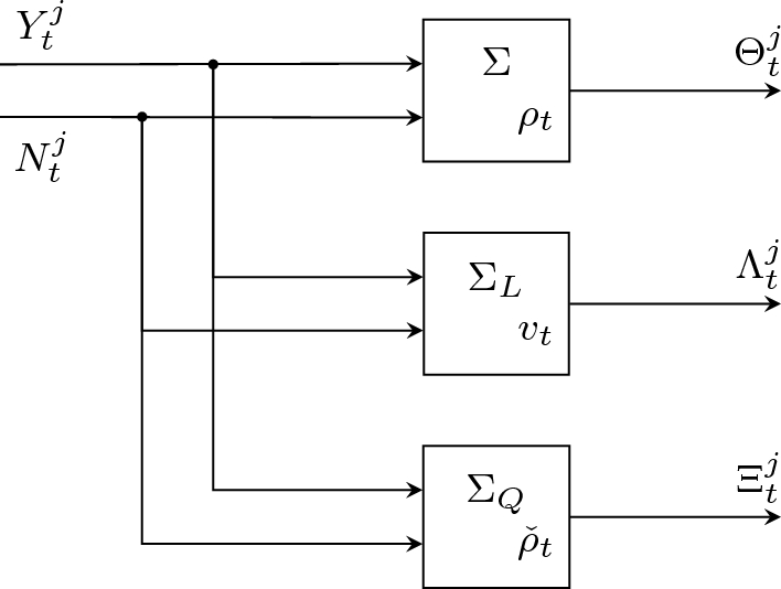
6.2.4 Numerical Simulations

In order to further test the validity of the reduced filter, we performed numerical simulations of the described model for \(N=4\). The numerical experiments have been performed as follows. Starting from a random initial condition \(\rho _0\) we simulated the stochastic evolution of the filter using the technique proposed by [59] and obtaining a realization of the quantum trajectory \((\rho _t)_\) as well as the measurement records \((Y_t^j)_\) and \((N_t^j)_\). Using the measurement records we then simulated the evolution of the original quantum filter starting from the initial condition \(\rho _0\) and the evolution of the reduced filter starting from the initial condition \(\check_0\) and computed the expectation values for the observables of interest \(\left\langle O_j(t) \right\rangle \) and for the local magnetization \(\langle }\rangle \). In Fig. 3 (first two rows) one can in fact observe that the population obtained in the standard basis \(\left\langle O_j(t) \right\rangle \) and local magnetization \(\langle \sigma _z^\rangle \) for both the full (dotted curves and empty circles) and reduced quantum model (continuous curves) are identical; hence, as expected, the reduced filter correctly reproduces the expectation of the observables of interest.

To conclude, since we have that \(\mathscr \) is \(\mathcal ^*\)-, \(\mathcal _D^*\)- and \(\mathcal _^*\)- invariant, Proposition 4 applies and hence \(\mathscr (\check_t,\check_t^e)-\mathscr (\rho _t,\rho _t^e)\ge 0\). This is depicted in the last row of Fig. 3 where the simulation has been run ten times with the original filter initialized in a random density operator \(\rho _0^e\) and the reduced filter has been initialized \(\check_0^e = \mathcal (\rho _0^e)\) while using the measurement records \((Y_t^j)_\) and \((N_t^j)_\) computed from the evolution of the original filter initialized in \(\rho _0\). One can see that the difference between the fidelity of the original model and that of the reduced one is always greater than 0. This shows that the reduced filter is less sensitive to initialization errors.