Existence and Uniqueness of Fixed Points Lemma A.1

For all \( |p | < \mu /2\) the map

$$\begin ( 0 ,\infty ) \ni x \mapsto \textstyle F( p, x) : = \mu \int \limits _} ^3 } | V (k) |^2 \big ( \mu \, \omega (k) - 2 p\cdot k + k^2 + x \big )^ \textrmk \end$$

(A.1)

has a unique fixed point \(F(p,x) = x\). Let \(g(p):=x\). Then, \(g \in C^1 ( \ )\).

Proof

Fix \(0< \varepsilon _0<1/2\) and let \(| p| \leqslant \varepsilon _0 \mu \). First, observe that

$$\begin \mu \omega (k) - 2 p\cdot k + k^2 + x \geqslant ( 1 - 2 \varepsilon _0) \mu |k | +x \qquad \forall x>0 \end$$

(A.2)

which follows from the reverse triangle inequality. Hence, thanks to our assumption on V we have \(F (p,x) \leqslant C \) for a constant \(C>0\) and all \(x>0\). Thus, F is well-defined. Next, note \( F (p,0) >0 \) (for otherwise V is equivalently zero). In addition, the map \(x\mapsto F(p,x)\) is \(C^1\). Indeed, one may compute directly

$$\begin \partial _x F (p,x)= - \mu \int \limits _} ^3} |V(k)|^2 \left( \mu \omega (k) -2 p \cdot k + k^2 +x \right) ^ d k \end$$

(A.3)

which is finite on \( | p |\leqslant \varepsilon _0\mu \) due to the lower bound of the denominator (A.2), and continuity follows from the monotone convergence theorem. On the other hand, the monotone convergence theorem implies \(\lim _ F(p,x )= 0\). Thus, the intermediate value theorem shows there exists at least one \(x \in (0, \infty )\) such that \( x - F(p,x) = 0 \). Further, note \( \partial _x F <0\). Thus, \( x\mapsto F (p,x ) \) is strictly decreasing. Therefore, the fixed point x must be unique. We then set \(g(p) = x. \) Finally, since \(x \mapsto F(p,x) \) is \(C^1\) on \( |p|< \varepsilon _0\mu \), the implicit function theorem implies that \(p\mapsto g(p)\) is \(C^1\) on \(\\). Since \(\varepsilon _0\) can be made arbitrarily close 1/2, this shows that g(p) is \(C^1\) on \( \\mu \} \). \(\square \)

We now establish the proof for the higher-order terms. Recall that for \( j\in \mathbb \) we let

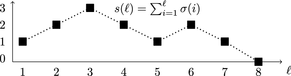
$$\begin \Sigma _0 ( j )&= \textstyle \^j \ : \ \sum _^ \sigma (i) \geqslant 1 \ \forall \ell \leqslant j -1 \ \ \text \ \ \sum _^j \sigma (i) = 0 \} \end$$

(A.4)

and we remind the reader of our notation \(b^_k = b^*_k\) and \(b^} = b_k\).

Lemma A.2

Let \( n\in \mathbb \). For all \( |p| < \mu /2 \) define the map on \( ( 0, \infty )\)

$$\begin x\mapsto F_n( p, x) = \sum _ J =2 \\ J \text \end }^ \sum _&\mu ^ \int \limits _} ^} \textrmk_1 \cdots \textrmk_ V(k_1) \cdots V(k_ ) \, \langle \Omega , b_}^} \ldots b_^} \Omega \rangle \nonumber \\ \textstyle&\times \prod _^ \bigg ( \mu \sum _^\ell \sigma (i) \omega (k_i) + \Big ( p - \sum _^\ell \sigma (i) k_i \Big )^2 - p^2 + x \bigg )^\ . \end$$

(A.5)

Then, there is a unique fixed point \( x = F_n(p,x)\). In addition, the map \(g_n(p) =x\) is \(C^1 ( \ )\).

Proof

Before we turn to the proof, let us briefly generalize Lemma A.1. Namely, let \(}\) be any finite set, and assume that for all \(s \in }\) we have a function

$$\begin F_s : B_r \times ( 0 , \infty ) \rightarrow ( 0 , \infty ) \end$$

where \(B_r = \} ^3: |p|<r \}\) . Further, assume that for all \( p \in B_r\) the map \(x\mapsto F_s(p,x)\) satisfies:

$$\begin \lim _ F_s(p,x)>0 \ , \quad F_s(p, \cdot ) \in C^1 ( 0 ,\infty ) \ , \quad \partial _x F_s (p, x) <0 \ , \qquad \lim _ F_s(p, x)=0 \ . \end$$

(C1)

Then, a repetition of the same argument presented for Lemma A.1 applies to the sum

$$\begin F_} }(p,x ) = \sum _ F_s( p, x ) \end$$

and we see that for all \( p \in B_r\) there is a unique fixed point \( x = F_}} (p,x)\). In addition, the map \(p \mapsto g(p) =x \) is of class \(C^1 (B_r). \)

Thus, in order to prove the claim of the present lemma, it suffices to fix an even integer \( J = 2 m \in \ \) and a permutation element \(\sigma \in \Sigma _0( J )\), and prove that the integral in (A.5) verifies the conditions (C1) with respect to (p, x). To this end, we consider the following measure on \( } ^\)

$$\begin d\nu _ (k_1, \ldots , k_J) : = V(k_1) \cdots V(k_ ) \, \langle \Omega , b_}^} \ldots b_^} \Omega \rangle d k_1 \ldots d \ . \end$$

(A.6)

Note that because \(\sum _\sigma (i)=0\), there is an equal number of indices satisfying \(\sigma (i) = \pm \). Let \( k_, \dots , k_\) be the momenta corresponding to the creation operators, that is, \(\sigma (i_\ell )= +1\). Likewise, let \( k_, \ldots , k_\) be the momenta corresponding to the annihilation operators with \(\sigma (j_\ell ) =-1\). Using the commutation relations \( [b_k, b^*_\ell ] = \delta ( k - \ell )\) and \(b_k\Omega =0\) we find that there is a subset S of the group of permutations of \(\\) such that

$$\begin d\nu _ (k_1, \ldots , k_J )&= \sum _ |V ( k_)|^2 \cdots |V ( k_)|^2 \delta ( k_ - k_ } )\nonumber \\&\cdots \delta (k_ - k_} ) d k_1 \ldots d . \end$$

(A.7)

The set S has the following property. Namely, it allows for contractions only for which

$$\begin i_1< j_ \ , \qquad i_2< j_ \ , \qquad \ldots \qquad i_m < j_ \ . \end$$

(A.8)

This is a consequence of the fact that we obtain the contractions by commuting the annihilation operators \(b_}\) to the creation operators \(b_^*\) to their right.

Because of the same reduction introduced above, it is sufficient to analyze the measure corresponding to a single permutation \(\gamma \in S\). We denote this measure by \(d \nu _^\gamma \) so that \(d \nu _ = \sum _ d \nu _^\gamma \). Integration of the function \(\prod _ ( \cdots )^\) in (A.5) yields

$$\begin F_^\gamma (p,x)&: = \int \limits _} ^} d\nu ^\gamma _ (k_1, \ldots , k_J)\prod _^ \big ( \cdots \big )^ \\&= \int \limits _} ^} d k_ \cdots d k_ |V ( k_)|^2 \ldots |V ( k_)|^2 H_\gamma ( k_, \ldots , k_ ) \end$$

where (for simplicity, we make the dependence on (p, x) implicit)

$$\begin H_\gamma ( k_, \ldots , k_ ) = \int \limits _} ^} d k_ \ldots d k_ \delta ( k_ - k_ } ) \ldots \delta (k_ - k_} ) \prod _^ \big ( \ldots \big )^ \ . \end$$

(A.9)

and we denote

$$\begin (\ldots )&= \mu \sum _^\ell \sigma (i) \omega (k_i) + \Big ( p - \sum _^\ell \sigma (i) k_i \Big )^2 - p^2 + x \nonumber \\&= \sum _^\ell \sigma (i) \Big ( \omega (k_i) - \mu p \cdot k_i \Big ) +\bigg ( \sum _^\ell \sigma (i) k_i \bigg )^2 + x \nonumber \\&= \sum _ 1\leqslant i \leqslant \ell \\ \sigma (i) =1 \end} \Big ( \omega (k_i) - \mu p \cdot k_i \Big ) - \sum _ 1\leqslant j \leqslant \ell \\ \sigma (j) = - 1 \end} \Big ( \omega (k_j) - \mu p \cdot k_j \Big ) + \bigg ( \sum _^\ell \sigma (i) k_i \bigg )^2 + x \ . \end$$

(A.10)

The contractions coming from the delta functions \(\delta (k_ - k_j)\) in (A.9) force cancelations between the positive and negative sums in (A.10). In particular, let us observe that thanks to (A.8) each of the \(k_j\) momenta with \(\sigma (j)=-1\) cancels one of the \(k_i \) moment, with \( i<j\). These \(k_i\) momenta are always included in the first sum (A.10) and therefore cancel out all the \(\sigma (j)=-1\) terms. However, since \(\sigma \in \Sigma _0(j)\) we have that \( \sum _ \sigma (i) \geqslant 1 \) for all \(1 \leqslant \ell \leqslant j-1\). That is, there is always at least one more \(\sigma =+\) index in the previous sum. This means that for any \(1 \leqslant \ell \leqslant j-1\) there is a non-empty set \(T(\ell ) \subset \\) of indices with \(\sigma =+\) such that

$$\begin H_\gamma ( k_, \ldots , k_ ) = \prod _^ \Big (\textstyle \sum _ \big ( \omega (k_) - \mu p \cdot k_i \big ) + \big ( \sum _^\ell \sigma (i) k_i \big )^2 + x \Big )^ \ . \end$$

(A.11)

With this representation we can repeat the argument in the proof of Lemma A.1 and verify that \(F_^\gamma (p,x) \) satisfies (C1). Thanks to the previous reductions, this finishes the proof. \(\square \)

Effective Dynamics for Massless Fields: Revisited

In this section, we consider massless models and iterate the algorithm in the proof of Theorem 2.2 one more time. Our goal is twofold. First, we show for the Nelson model that it is possible to improve the time scale given by Theorem 2.2 by a logarithmic factor. Secondly, we study massless models whose form factors are less singular than the Nelson model.

The following family of models serves as an archetype for both situations

$$\begin V_a(k) = |k|^ \mathbbm (|k |\leqslant \Lambda ) \ , \end$$

(B.1)

where \(a \in [0,1/2]\). It will be convenient to introduce the following scale of norms, quantifying infrared behavior

$$\begin |\hspace|\hspace|V |\hspace|\hspace|_ : = \Vert \omega _\mu ^ V \Vert _ \ , \qquad s>0 \ . \end$$

(B.2)

Note that our old norm fits into this scale as follows \(\Vert V \Vert _ = \Vert V \Vert _\). The reader should keep in mind that the following estimates hold for the models (B.1)

$$\begin&\Vert V_a \Vert _ \leqslant C (\log \mu )^ & \text & \Vert V_a\Vert _ \leqslant C \mu & \text a = 1/2 \end$$

(B.3)

$$\begin&\Vert V_a \Vert _ \leqslant C & \text & \Vert V_a \Vert _ \leqslant C \mu ^+a} & \text a \in [0,1/2) \ . \end$$

(B.4)

In our next theorem, we study the dynamics of massless fields and obtain an approximation that is valid over slightly longer time scales, in comparison to the results of Theorem 2.2. In order to keep the next statement to a reasonable length, we have chosen to consider only the form factors given by (B.1), although our results apply to more general interactions if one wishes to keep track of the norms \(\Vert V\Vert _\).

Theorem B.1

Let \(\omega (k)=|k|\) and \( V = V_a\) as in (B.1) with \( a \in [0,1/2]\). Let \(\Psi _0\) satisfy Condition 1. Then, there exists a constant \(C>0\) such that for all \(t \in } \) and \(\mu >0\) large enough

$$\begin&\Vert \Psi (t) - \Psi _\text (t) \Vert _} \leqslant C \bigg ( \frac \bigg )^ (1 + |t|) & \text a = 1/2 \ , \end$$

(B.5)

$$\begin&\Vert \Psi (t) - \Psi _\text (t) \Vert _} \leqslant \frac} (1 + |t|) & \text a \in [0,1/2) \ . \end$$

(B.6)

Remark B.1

Let us now comment on the consequences that Theorem B.1 has for the observed time scales.

(1)

For \(a = \frac\) (the massless Nelson model) we have an effective approximation for time scales

$$\begin \, | t | \, \ll \Big ( \frac \Big )^ \end$$

which improves the result of Theorem 2.2 by a factor \((\log \mu )^\frac\).

(2)

For \( 0 \leqslant a < \frac\) we have an effective approximation for time scales

$$\begin \, | t | \, \ll \mu ^\ \end$$

which improves the result of Theorem 2.2 by a factor \(\mu ^. \)

(3)

The reader may wonder if it possible to extend the massless approximation to even longer time scales. Currently, our methods do not allow for such an extension unless one introduces a suitable infrared cutoff on the interaction potential V. In particular, we cannot prove a result similarly to Theorem 2.4 for the massless case.

Let us recall that \(}= }^+ + }^-\) is the interaction term (2.2), and \( } \) is the resolvent operator (3.7).

Proof

Similarly as in the proof of Theorem 2.2, we consider

$$\begin \Vert \Psi (t) - \Psi _\text (t)&\Vert \leqslant \Vert }(t) } }\Psi _0 \Vert + \Vert }(t) \textbf _\Omega } } }\Psi _0 \Vert \nonumber \\&\leqslant \frac|\hspace|V |\hspace|\hspace|_\mu }} + \Vert }(t) \textbf _\Omega } } }\Psi _0 \Vert , \end$$

(B.7)

where we have employed Proposition 4.1 to estimate the first boundary term. Our next goal is to give a more precise estimate of the error term

$$\begin }(t) \equiv }(t) \textbf _\Omega } } }\Psi _0 = }(t) }^+ } }^+ \Psi _0 \ , \end$$

(B.8)

where in the second line we have kept only the nonzero contributions. Making use of the integration-by-parts formula (4.1), we find

$$\begin }(t)&= }(t) }^+ } }^+ \Psi _0 \nonumber \\&= \Big ( }(t) } + }(t) } } \Big ) }^+ } }^+ \Psi _0 \nonumber \\&= }(t) } }^+ } }^+ \Psi _0 + }(t) } } }^+ } }^+ \Psi _0 \nonumber \\&= }(t) } }^+ } }^+ \Psi _0 + }(t) }^+ } }^+ } }^+ \Psi _0 + }(t) }^- } }^+ } }^+ \Psi _0 \ . \end$$

(B.9)

Observe that the last term of the right-hand side of (B.9) contains an operator \(}^-\). This has the effect of introducing contractions between creation and annihilation operator, which lead to worse infrared behavior. However, these are still one-particle states and may be integrated by parts one more time. Namely, we find

$$\begin }(t)&= }(t) } }^+ } }^+ \Psi _0 + }(t) }^+ } }^+ } }^+ \Psi _0+ }(t) } }^- } }^+ } }^+ \Psi _0 \nonumber \\&\quad + }(t) } } }^- } }^+ } }^+ \Psi _0 \nonumber \\&= }(t) } }^+ } }^+ \Psi _0 + }(t) }^+ } }^+ } }^+ \Psi _0+ }(t) } }^- } }^+ } }^+ \Psi _0 \nonumber \\&\quad + }(t) }^+ } }^- } }^+ } }^+ \Psi _0 + }(t) }^- } }^- } }^+ } }^+ \Psi _0 \end$$

(B.10)

where in the last line we decomposed \(}= }^+ + }^-\). Next, we make use of the observation form Remark 4.3, as well as the bounds \( \Vert }(t )\Vert \leqslant 2 \) and \(\Vert }(t)\Vert \leqslant |t|\) to find that

$$\begin \Vert }(t)\Vert&\leqslant C \Vert } }^+ } }^+ \Psi _0 \Vert + C (1 + \, \mu ^| t | ) \Vert } }^+ } }^+ } }^+ \Psi _0 \Vert + C\Vert } }^- } }^+ } }^+ \Psi _0 \Vert \nonumber \\&+ C (1 + \, \mu ^ |t | ) \Vert } }^+ } }^- } }^+ } }^+ \Psi _0 \Vert + C \, | t | \, \Vert }^- } }^- } }^+ } }^+ \Psi _0 \Vert \end$$

(B.11)

for some constant \(C>0\). All the terms in the expansion for \(}(t)\) are separately estimated in Proposition B.1. The proof of the theorem is finished once we gather these estimates back in (B.7) and use (B.3) to collect the leading order terms in the two different regimes for \( a \in [0,1/2]\). \(\square \)

Proposition B.1

There is a constant \(C>0\) such that the following five estimates hold.

(i)

\(\Vert } }^+ } }^+ \Psi _0\Vert _} \leqslant C\mu ^ |\hspace|\hspace|V |\hspace|\hspace|^2_ \)

(ii)

\( \Vert } }^+ } }^+ } }^+ \Psi _0 \Vert _} \leqslant C \mu ^ |\hspace|\hspace|V |\hspace|\hspace|_^3 \)

(iii)

\( \Vert } }^- } }^+ } }^+ \Psi _0 \Vert _} \leqslant C \mu ^ |\hspace|\hspace|V |\hspace|\hspace|_ |\hspace|\hspace|V |\hspace|\hspace|_^2 \)

(iv)

\(\Vert } }^+ } }^- } }^+ } }^+ \Psi _0 \Vert _} \leqslant C \mu ^ |\hspace|\hspace|V |\hspace|\hspace|_ |\hspace|\hspace|V |\hspace|\hspace|_ |\hspace|\hspace|V |\hspace|\hspace|_^2 \)

(v)

\( \Vert }^- } }^- } }^+ } }^+ \Psi _0 \Vert _} \leqslant C \mu ^ |\hspace|\hspace|V |\hspace|\hspace|_^2 |\hspace|\hspace|V |\hspace|\hspace|_^2 \ . \)

In the following proof we will make use of the estimates in Sect. 7 that were developed for massive fields, but apply here as well as long as no mass terms appear. See Remark 7.3. We also use the notation for resolvents \(R_p(k)\), \(R_p(k_1, k_2)\), etc., introduced in Sect. 7.1.

Proof of Proposition B.1

(i) Apply (7.7) with \(n=2\).

(ii) Apply (7.7) with \(n=3 \).

(iii) The state can be calculated explicitly using standard commutation relations as well as the contraction of the field operators \( b_ b_^* b_^* \Omega = \delta (k_3 - k_2) b_^* \Omega + \delta (k_3 - k_1) b_^* \Omega \). We find that (here \(\int = \int _} ^} \textrmk_1 \textrmk_2\))

$$\begin } }^- } }^+ } }^+ \Psi _0&\, = \, \mu ^ \int V(k_1) | V(k_2) |^2 e^ R_p (k_1)^2 R_p ( k_1, k_2) \varphi \otimes b_^* \Omega \nonumber \\&+ \mu ^ \int | V(k_1) |^2 V(k_2) e^ R_p (k_1) R_p (k_2) R_p ( k_1, k_2) \varphi \otimes b_^* \Omega \nonumber \\&\quad \, =: \, \Phi _} _} \end$$

(B.12)

Here we have written the one-particle state \( } }^- } }^+ } }^+ \Psi _0 \) in terms of \(\Phi _} _}\) (see Definition 7.1) with coefficients

$$\begin } _ ( k_1,p) \ : = \ &\mu ^V(k_1)R_p (k_1)^2 \int |V(k_2)|^2 R_p(k_1,k_2) \textrmk_2 \nonumber \\&+ \mu ^ V(k_1)R_p (k_1) \int |V(k_2)|^2 R_p(k_2) R_p(k_1,k_2) \textrmk_2 \ . \end$$

(B.13)

Finally, we borrow estimates from Sect. 7. An application of (7.12) and (7.3) implies that

$$\begin \Vert } }^- } }^+ } }^+ \Psi _0 \Vert \leqslant \Vert } _ \Vert _ \leqslant C \mu ^ \Vert \omega _\mu ^ V \Vert _ \Vert \omega _\mu ^} V \Vert _^2 \ . \end$$

(B.14)

(iv) In the notation of (iii) and Lemma 7.2, we note that \( } }^+ } }^- } }^+ } }^+ \Psi _0 = } }^+ \Phi _} _} = \Phi _} _1^+ } \). Consequently,

$$\begin \Vert } }^+ } }^- } }^+ } }^+ \Psi _0 \Vert = \Vert \Phi _} _1^+ } \Vert \leqslant \Vert } _1^+ \Vert _ \leqslant C \mu ^ |\hspace|\hspace|V |\hspace|\hspace|_ \Vert } _} \Vert _\ . \end$$

(B.15)

It suffices to combine the previous estimate with (B.14) to finish the proof.

(v) We use the representation (B.12) and act on it with \(}^- = \int V(k) e^b_k \textrmk \) to find

$$\begin }^- } }^- } }^+ } }^+ \Psi _0 = \mu ^} \bigg ( \int \limits _} ^3} V(k) } _1( k,p) \textrmk \bigg ) \varphi \otimes \Omega \ . \end$$

(B.16)

Next, we note that for all \(|p| \leqslant \varepsilon \mu \) we may estimate thanks to the explicit expression (B.13) and the resolvent estimates (7.3):

$$\begin \bigg \Vert \int \limits _} ^3} \mu ^ V(k) } _1 ( k,p) \textrmk \bigg \Vert \leqslant \frac |\hspace|\hspace|V |\hspace|\hspace|_^2 |\hspace|\hspace|V |\hspace|\hspace|_^2 \ . \end$$

(B.17)

The proof is then finished once we combine the last two displayed estimates. \(\square \)

The Generator and the Fiber Hamiltonians

The goal of this section is to establish the asymptotic relationship between the effective dispersion relation \(\text _(p)\) and the energy–momentum relation \(\inf \textrm H(p)\), as mentioned in (2.13). The energy–momentum relation is the infimum of the spectrum of the fiber Hamiltonians

$$\begin H(p) : = (p -P)^2 + T + V^+ + V^- \ , \qquad p\in } ^3 \end$$

(C.1)

where \( V^+ = \mu ^ b^*(V)\), \(V^- = \mu ^ b(V)\), \(T = \mu d \Gamma (\omega )\) and \(P = d \Gamma (k)\) are operators acting only on the bosonic Fock space \(\mathscr \). The fiber Hamiltonians are related to the original Hamiltonian through a direct integral decomposition \(H \cong \int _} ^3}^ H(p) d p\), which is obtained by transforming H with \(e^\) and then taking the Fourier transformation in x.

The main result of this section is the following theorem, where we focus on the massless case. To the best of our knowledge, this result is new. For comparison, a related (non-asymptotic) result for H(p) when restricted to the subspace of less than two field excitations was established in [7].

Theorem C.1

Let \(\omega (k) = |k| \) and assume that \( V(k) = \mathbbm (|k|\leqslant \Lambda ) \omega (k)^\). Let g(p) be the solution to (2.8). Then, for every \(\varepsilon \in [ 0,1/2)\) there exists a constant \(C>0\) such that for all \(| p| \leqslant \varepsilon \mu \) and \(\mu \) large enough:

$$\begin - \frac \ \leqslant \ \inf \textrm H(p) - \left( p^2 - g(p) \right) \ \leqslant \ \frac \ . \end$$

(C.2)

Before proving the theorem, let us highlight its non-trivial implications for the energy–momentum relation, particularly in the momentum regime \(|p| \sim \mu \).

Corollary C.1

Let \(\omega \) and V as in Theorem C.1. For all \(|p|< \frac\), the energy–momentum relation satisfies

$$\begin \lim _ \left( \inf \textrm H(\mu p) - (\mu p)^2 \right) = \frac \tanh ^ (2|p|) \int \limits _} ^3 } \frac dk . \end$$

(C.3)

We will prove Theorem C.1 in a slightly more general setting. Let us recall the definition of the norm \(|\hspace|\hspace|V |\hspace|\hspace|_\mu \equiv \Vert \omega _\mu ^ V \Vert _\) with \(\omega _\mu = \omega + \mu ^\). We assume that V verifies Condition 1 and, in addition, that

$$\begin |\hspace|\hspace|V |\hspace|\hspace|_\mu ^2 \ll \mu \quad \text \quad \mu \gg 1 \ . \end$$

(C.4)

Proof of Theorem C.1

We fix \(\varepsilon \in [0,\frac)\) and \(|p| \leqslant \varepsilon \mu \). First we establish an upper bound via the trial state

$$\begin \Psi (p) = (1 + R (p) V^+ )\Omega \in \mathscr , \end$$

(C.5)

where we introduced \(R(p):= ( - g(p) + p^2 - (p-P)^2 -T )^\). Using \(T\Omega = 0 = P\Omega \), and that \( R (p) V^+ \Omega \in \text ( \textbf _\Omega )\) with \( \textbf _\Omega = \mathbbm - |\Omega \rangle \langle \Omega |\), a straightforward calculation gives

$$\begin&\left\langle \Psi (p) , \left( H(p) - p^2 \right) \Psi (p) \right\rangle _\mathscr = 2 \left\langle \Omega , V^- R(p) V^+ \Omega \right\rangle _\mathscr \nonumber \\&\qquad \qquad \qquad + \left\langle \Omega , V^- R(p)\left( (p-P^2) - p^2 + T + V^+ + V^- \right) V^+ R(p) \Omega \right\rangle _\mathscr . \end$$

(C.6)

In the second line, we use that the terms cubic in \(V^\pm \) vanish and then add \(g(p) \geqslant 0\) inside the brackets, so that

$$\begin \left\langle \Psi (p) , \left( H(p) - p^2 \right) \Psi (p) \right\rangle _\mathscr &\leqslant \left\langle \Omega , V^- R(p) V^+ \Omega \right\rangle _\mathscr \nonumber \\&= - \int \frac = -g(p). \end$$

(C.7)

Next, we observe that \(\Vert \Psi (p)\Vert ^2_\mathscr = 1 + \Vert R(p) V^+ \Omega \Vert ^2 \leqslant 1 + C \mu ^ |\hspace|\hspace|V |\hspace|\hspace|_\mu ^2\) which follows by the same argument as in the proof of Proposition 4.1. Thus, by assumption that \(\mu ^ |\hspace|\hspace|V |\hspace|\hspace|_\mu ^2 \ll 1\), we have \(\Vert \Psi (p)\Vert ^_\mathscr \geqslant 1 - C \mu ^ |\hspace|\hspace|V |\hspace|\hspace|_\mu ^2\). Combining the above and invoking the variational principle for the ground state energy, we arrive at

$$\begin \inf \textrm H(p) \leqslant \frac}} \leqslant p^2 - g(p) + C \frac|\hspace|V |\hspace|\hspace|_\mu ^2} g(p). \end$$

(C.8)

The proof of the upper bound is concluded by using \(0 \leqslant g(p) \leqslant C_1\) for some (\(\varepsilon \)-dependent) constant \(C_1>0\).

Now we prove the lower bound. Here, the main step is to complete the square in the following fashion

$$\begin \int \left( f(k) b_k^*b_k + \overline (k) b_k + w(k) b_k^* \right) d k \geqslant - \int \frac dk \end$$

(C.9)

for suitable functions \(f> 0\) and w. This inequality is understood in the sense of quadratic forms on \( Q ( H(p) ) \subset Q(T) \cap Q(P^2) \subset \mathscr \). We choose \(w(k) = \mu ^ V(k)\) and \(f(k) = \mu \omega (k) - 2 p\cdot k\) and recall that \(\mu \omega (k) - 2 p\cdot k \geqslant \mu \omega (k) (1-2\varepsilon ) > 0\). This gives the lower bound

$$\begin H (p) \geqslant (p-P)^2 + T - d\Gamma ( f ) - \int \frac \ . \end$$

(C.10)

The last term can be compared to g(p) with remainder estimate

$$\begin \int \frac - g(p)&\leqslant \int \frac \nonumber \\&\leqslant C g(p) \mu ^ \Vert \omega ^ \omega _\mu ^ V \Vert _^2 + C \mu ^ \Vert V \Vert _^2. \end$$

(C.11)

Since \(d\Gamma (f) = T - 2 p\cdot P\), we can bound the other terms in (C.10) as

$$\begin (p-P)^2 + T - d\Gamma (f)&= p^2 + P^2 \geqslant p^2 . \end$$

(C.12)

Combining these three inequalities leads to the desired lower bound:

$$\begin H(p) \geqslant p^2 - g(p) - C \mu ^ \Vert \omega ^ \omega _\mu ^ V \Vert _^2 - C \mu ^ \Vert V \Vert _^2. \end$$

(C.13)

In order to finish the proof, we combine the upper and lower bounds to find that for all \( |p |\leqslant \varepsilon \mu \)

$$\begin - \frac \left( \Vert \omega ^ \omega _\mu ^ V \Vert _^2 + \Vert V \Vert _^2 \right) \ \leqslant \ \inf \textrm H(p) - \left( p^2 - g(p) \right) \ \leqslant \ \frac |\hspace|\hspace|V |\hspace|\hspace|_\mu ^2 . \end$$

(C.14)

The proof of the theorem is finished after we use the following bounds for Nelson model \(V(k) = \mathbbm ( |k |\leqslant \Lambda ) \omega (k)^\), namely that \(|\hspace|\hspace|V |\hspace|\hspace|_\mu ^2 \leqslant \Vert \omega ^ \omega _\mu ^ V \Vert _^2 \leqslant 4\pi \log (\mu \Lambda + 1)\). \(\square \)

Proof of Corollary C.1

We use Theorem C.1 and Corollary 5.1 with \(p\rightarrow \mu p \) (for \(\mu |p| < \frac\)), and then apply monotone convergence to obtain the limit

$$\begin \lim _ \int \limits _} ^} \frac \tanh ^ \bigg ( \frac \bigg ) \ \textrmk = \tanh ^ (2|p|) \int \frac \textrmk . \end$$

(C.15)

This finishes the proof. \(\square \)