Mathematical notation

 

We denote matrices and datasets with bold capital letters: \(\varvec\)

If \(\varvec\) denotes a matrix, we introduce it as \(\varvec = \left[ y_\right] \in \mathbb ^\) for which:

there are N rows and D columns

\(y_\) denotes the value in the nth row and the dth column

\(\varvec_\) denotes the nth row vector, and \(\varvec_\) denotes the dth column vector

If \(\varvec\) denotes a dataset comprised of multiple matrices, we specify this, and denote each of the matrices as \(\varvec^ = \left[ y_^\right] \in \mathbb ^\)

We denote parameters for statistical distributions as non-bold, lower case letters. If the parameter is for a random variable stored in a matrix, we add indices. For example, \(\tau _^\) is a parameter for a random variable in the nth row and dth column of the mth matrix of some dataset. If \(\tau _^\) is a parameter for the same matrix, then it is used for all values in the dth column.

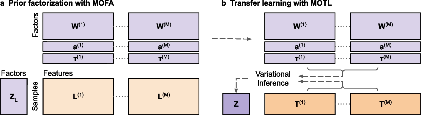
The MOFA model

Consider a multi-omics dataset \(\varvec\) consisting of omics matrices \(\varvec^\), \(m=1,...,M\). Each \(\varvec^ = \left[ y_^\right] \in \mathbb ^\) contains data for N samples (rows) and \(D_m\) features (columns), where \(y_^\) is the value for the nth sample and the dth feature from the mth matrix. MOFA [44], assumes the existence of latent factors, and jointly factorizes each \(\varvec^\) into a shared matrix of sample scores \(\varvec = \left[ z_\right] \in \mathbb ^\), and an omics specific matrix of feature weights \(\varvec^ = \left[ w_^\right] \in \mathbb ^\). The kth column of \(\varvec\) contains scores for the kth factor, and the kth row of \(\varvec^\) contains corresponding weights for that factor.

MOFA assumes that each observed \(y^_\) is a random variable, characterized by a probability distribution conditional on a set of latent random variables \(\varvec\). It is assumed that the joint likelihood \(p(\varvec|\varvec)\) is equal to \(\overset} \ \overset} \ \overset}} \ p(y_^ \ | \ \varvec)\), and the choice of probability distribution depends on the type of observed data. A Gaussian likelihood is assumed for observed continuous data:

$$\begin p(y_^ \ | \ \varvec) = \text \left( y_^ \ | \ \varvec_ \varvec_^ , 1/ \tau _^ \right) \end$$

(7)

where \(\varvec_\) is the vector of scores for the nth sample, \(\varvec_^\) is the vector of weights the dth feature from the mth matrix, and \(\tau _^\) is the precision for that feature. A Bernoulli likelihood is assumed for observed binary data and the logistic link function \(\pi (x) = (1+e^)^\) is used:

$$\begin p(y_^ \ | \ \varvec) = \text \left( y_^ \ | \ \pi \left( \varvec_ \varvec_^\right) \right) \end$$

(8)

A Poisson likelihood is assumed for observed counts data and the link function \(\lambda (x)=\text (1+e^x)\) is used:

$$\begin p(y_^ \ | \ \varvec) = \text \left( y_^ \ | \ \lambda \left( \varvec_ \varvec_^\right) \right) \end$$

(9)

The assumed joint prior distribution, \(p(\varvec)\), is comprised of independent priors: \(z_ \sim \text (0, \ 1)\), \(w_^ = \hat_^ s_^\), \(\hat_^ \sim \text (0, \ 1/ \alpha _k^)\), \(\alpha _k^ \sim \text (1e^, \ 1e^)\), \(s_^ \sim \text (\theta ^_k)\), \(\theta ^_k \sim \text (1, \ 1)\), \(\tau _^ \sim \text (1e^, \ 1e^)\).

MOFA uses mean-field variational inference [32, 45, 46] to approximate the joint posterior distribution, \(p(\varvec|\varvec)\), with a joint variational distribution factorized over J disjoint groups of variables:

$$\begin q(\varvec) & = \overset} q(\varvec_j) \nonumber \\ & = \overset} \ \overset} \ q(z_) \ \overset} \ \overset} \ q(\alpha _k^) \ q(\theta ^_k) \ \overset} \ \overset}} \ q(\tau _^) \ \overset} \ \overset}} \ \overset} \ q(\hat_^, s_^) \end$$

(10)

MOFA infers \(q(\varvec)\) iteratively until convergence. At each iteration, each \(q(\varvec_j)\) is updated as

$$\begin q(\varvec_j) \propto exp \_}[\log \ p(\varvec,\hat})] \} \end$$

(11)

where \(\mathbb _}\) denotes an expectation with respect to the joint variational distribution, after removing \(q(\varvec_j)\). The dataset \(\hat}\) is derived by transformation of \(\varvec\). Observed data with a Gaussian assumed likelihood are transformed with feature-wise centering, which avoids the need to estimate intercepts. Observed data with a non-Gaussian assumed likelihood are transformed to derive Gaussian pseudo-data. The derivation of Gaussian pseudo-data occurs at each iteration, and is based on a new parameter, \(\zeta _^\), which is derived for each sample n and feature d from matrix m. For observed data with a Bernoulli assumed likelihood, a precision parameter, \(\tau _^\), is introduced for each sample and feature as part of the transformation:

$$\begin \hat_^ = \frac^ - 1}^} \end$$

(12)

$$\begin \tau _^ = 2 \lambda \left( \zeta _^ \right) \end$$

(13)

$$\begin \left( \zeta _^ \right) ^2 = \mathbb _q \left[ \left( \varvec_ \varvec_^ \right) ^2\right] \end$$

(14)

For observed data with a Poisson assumed likelihood, a precision parameter, \(\tau _^\), is introduced for each feature as part of the transformation:

$$\begin \hat_^ = \zeta _^ - \frac^\right) \left( 1-y_^ / \lambda \left( \zeta _^ \right) \right) }^} \end$$

(15)

$$\begin \zeta _^ = \mathbb _q \left[ \varvec_ \varvec_^\right] \end$$

(16)

$$\begin \tau _^ = 0.25 + 0.17 \times max\left( \varvec_^\right) \end$$

(17)

where \(\varvec_^\) is the vector of observed values for the dth feature from the mth matrix. For both Bernoulli and Poisson observed data, the \(\hat_^\) values are centered at each iteration, and \(\zeta _^\) values are derived using the factorization fit from the preceding iteration. MOFA monitors convergence with the evidence lower bound (ELBO), which is used to evaluate how well the variational distribution approximates the posterior distribution. The ELBO is calculated as:

$$\begin \text (\varvec) = \mathbb _\left[ \text \ p(\varvec|\varvec)\right] + \mathbb _\left[ \text \ p(\varvec)\right] - \mathbb _\left[ \text \ q(\varvec)\right] \end$$

(18)

For \(\varvec^\) with non-Gaussian assumed likelihood, MOFA uses a lower bound for each \(\text \ p\left( y_^|\varvec\right)\). Maximizing this lower bound, coupled with the use of \(\hat_^\) values, allows updates of \(q(\varvec)\) based on the assumption of Gaussian observed data [33, 34]. MOFA assesses convergence at regular intervals, based on the percentage change in ELBO after. MOFA allows factors to be dropped during training, based on the fraction of variance explained for each matrix. After each iteration, MOFA identifies factors that do not explain a fraction of variance, for any omics matrix, over a threshold. MOFA then drops one of the identified factors.

Multi-omics data simulated with groundtruth factors

We simulated multi-omics datasets, from groundtruth factors, with various configurations. For each simulation configuration, we generated 30 instances of a multi-omics dataset, \(\varvec\), consisting of matrices, \(\varvec^, m = 1,2,3\). We split each \(\varvec\) into a target dataset, \(\varvec\), and a learning dataset, \(\varvec\). Each \(\varvec^ = \left[ y_^\right] \in \mathbb ^\) contained data for \(N=N_t + N_l\) samples (rows) and \(D_m = 2000\) features (columns), where \(y_^\) is the value for the nth sample and the dth feature from the mth matrix. \(N_t\) is the number of samples subsequently belonging to \(\varvec\), and \(N_l\) is the number of samples belonging to \(\varvec\). We generated each \(\varvec^\) from a different statistical distribution, conditional on a random matrix of sample scores, \(\varvec = \left[ z_\right] \in \mathbb ^\), and a random matrix of feature weights, \(\varvec^ = \left[ w_^\right] \in \mathbb ^\). The kth column vector of \(\varvec\) contained sample scores for the kth groundtruth factor. The kth row vector of \(\varvec^\) contained feature weights for that same factor. We varied the number of groundtruth factors across configurations, using \(K \in \\).

We generated \(\varvec\) based on each sample being a member of a group. In each instance we created two groups of five samples belonging to \(\varvec\), meaning \(N_t\) was always equal to 10 samples. We allowed \(N_l\) to vary across instances, with samples belonging to \(\varvec\) being in differently sized groups of randomly selected sizes. We used either 20 learning groups of size \(\in \\), or 40 groups of size \(\in \\). For the nth sample and kth groundtruth factor, we generated the score as \(z_ \sim \text (\mu _, \ \sigma _z)\), where \(\mu _\) is the mean parameter for groundtruth factor k, for the group that sample n belonged to, g(n). In each instance we selected \(\mu _\) randomly for each group and groundtruth factor, with probabilities \(Pr(3) = 1/8\), \(Pr(5) = 3/4\), \(Pr(7) = 1/8\). The kth groundtruth factor was differentially active for \(\varvec\) if \(\mu _\) differed between the two target dataset groups. For all instances of a given simulation configuration, the same standard deviation parameter, \(\sigma _z\), was shared by all groups and groundtruth factors. We varied the latent noise-to-signal ratio across our simulation configurations by using \(\sigma _z \in \\).

For the kth groundtruth factor, and the dth feature from the mth matrix, we generated the weight as \(w_^ = \hat_^ s_^\). As such, each \(w_^\) was the product of a continuous random variable, \(\hat_^ \sim \text (\mu ^, \ \sigma _^)\), and a binary random variable, \(s_^ \sim \text (\theta ^_k)\). We specified \(\mu ^\), the mean parameter for the mth matrix, with \(\mu ^ = 5\); \(\mu ^ = 0\); \(\mu ^ = 0\). We generated, \(\sigma _^\), the standard deviation parameter for the kth groundtruth factor and the mth matrix, with \(\sigma _^ \sim \text (0.5, 1.5)\); \(\sigma _^ \sim \text (0.5, 1.5)\); \(\sigma _^ \sim \text (0.1, 0.2)\). We generated the sparsity for the kth groundtruth factor and the mth matrix, \(1 - \theta ^_k\), with \(\theta ^_k \sim \text (0.15, 0.25)\).

We generated the values in each \(\varvec^\) as:

$$\begin y_^ & \sim \text \left( \text \left( 1 + \text \left( \varvec_ \varvec_^\right) \right) \right) \nonumber \\ y_^ & \sim \text \left( \varvec_ \varvec_^, \ \sigma _d \sim \text \left( 0.25, 0.75\right) \right) \nonumber \\ y_^ & \sim \text \left( 1/\left( 1 + \text \left( -\varvec_ \varvec_^\right) \right) \right) \end$$

(19)

where \(\varvec_\) is the vector of scores for the nth sample, \(\varvec_^\) is the vector of weights the dth feature from the mth matrix, and \(\sigma _d\) is the standard deviation for the dth feature.

We split each \(\varvec^\) into \(\varvec^ = \left[ t_^\right] \in \mathbb ^\), which contained values for the target group samples, and \(\varvec^ = \left[ l_^\right] \in \mathbb ^\), which contained values for the learning group samples.

Before direct factorization with MOFA we pre-processed simulated \(\varvec\) and \(\varvec\) datasets by removing features with 0 variance across samples. Before factorization with transfer learning with MOTL, we pre-processed simulated \(\varvec\) datasets by removing features that had 0 variance across samples or that had been removed from the corresponding \(\varvec\) datasets.

TCGA multi-omics data acquisition and pre-processing

We used the R packages TCGAbiolinks (v.2.25.3) and SummarizedExperiment (v.1.28.0) to download and save TCGA mRNA expression, miRNA expression, DNA methylation, and simple nucleotide variation (SNV) data [47,48,49]. The mRNA and miRNA expression data consisted of raw counts. The DNA methylation data consisted of CpG site \(\beta\)-values, which had been derived from HM450 array intensities with R package SeSAMe (v.1.16.0) [50]. The SNV data consisted of masked somatic mutation files.

We created four reference datasets, using data from three cancer types; acute myeloid leukemia (LAML), pancreatic adenocarcinoma (PAAD) and skin cutaneous melanoma (SKCM). Each reference dataset, \(\varvec\), contained multi-omics data for all samples from either two, or all three of the cancer types. We did not include SNV data in \(\varvec\) datasets containing LAML samples, due to the sparsity of SNV data for LAML. We only used samples that had data for all omics of interest, and only included one sample per study participant. We thus had multi-omics data for 134 LAML samples, 157 PAAD samples, and 435 SKCM samples. We then randomly split each \(\varvec\) into non-overlapping target datasets. Each resulting target dataset, \(\varvec\), contained multi-omics data for five samples per cancer type.

For the evaluation protocol based on TCGA multi-omics data, we merged data from the remaining 29 cancer types into a learning dataset, \(\varvec\). For this \(\varvec\), we only used samples that had data for all four omics, and only included one sample per study participant. This \(\varvec\) contained multi-omics data (mRNA, miRNA, DNA methylation, and SNV) for 7217 samples.

For the application of MOTL to the pd-GBSC target datasets, we created a new learning dataset by merging data from all 32 cancer types. This new learning dataset contained multi-omics data (mRNA, miRNA, DNA methylation, and SNV) for 7866 samples.

Before direct factorization with MOFA, we pre-processed \(\varvec\), \(\varvec\), and \(\varvec\) datasets in the same way. For mRNA data, we removed genes that map to the Y chromosome. For both mRNA and miRNA, we removed genes if they had a count of zero in \(\ge 90\%\) of samples, or had zero variance across samples. We normalized mRNA and miRNA counts with the DESeq2 (v.1.38.0) R package [51], and \(\text _2(x+1)\) transformed the normalized counts. For DNA methylation data, we removed CpG sites that map to the X or Y chromosome, were masked during SeSAMe quality control, had missing values in \(\ge 20\%\) of samples, or had zero variance across samples. We converted DNA methylation \(\beta\)-values to M-values [52]. We included SNV records whose variant classification was either Frame_Shift_Del, Frame_Shift_Ins, In_Frame_Del, In_Frame_Ins, Missense_Mutation, Nonsense_Mutation, Nonstop_Mutation, Splice_Site, or Translation_Start_Site. We then created binary SNV matrices aggregated by gene and sample. We removed genes from SNV matrices if the mutation rate across samples was \(\le 1\%\). We filtered all omics to include only the 5000 most variable features. We did not perform any batch effect correction on \(\varvec\) datasets in order to preserve biological signal [53]. We checked each \(\varvec\) for batch effects with visualizations of UMAP co-ordinates [54]. We used the R package uwot (v.0.1.14) to derive UMAP coordinates from MOFA factorizations, and we did not observe the need to correct \(\varvec\) datasets for batch effects.

Before factorization with transfer learning with MOTL, we pre-processed \(\varvec\) datasets by removing all omics features that had zero variance across samples, or that had been removed from \(\varvec\) during pre-processing. We used DESeq2 to normalize mRNA and miRNA counts with the geometric means from \(\varvec\), and then \(\text _2(x+1)\) transformed the normalized counts. We converted DNA methylation \(\beta\)-values to M-values, and converted SNV data to binary matrices after filtering on variant classification, as described previously.

Glioblastoma target dataset acquisition and pre-processing

We created four pd-GBSC target datasets, based on multi-omics profiling conducted by Santamarina-Ojeda et al. [36] for four normal brain samples and nine patient-derived glioblastoma stem cell (pd-GBSC) cultures. The nine cancer samples had been previously classified into three subtypes thanks to transcriptome-based signatures: classical (CL), proneural (PN), and mesenchymal (MS). Each pd-GBSC target dataset contained mRNA expression and DNA methylation data for the four normal brain cortex samples, as well as either all nine cancer samples or just the samples from a subtype.

For factorization with transfer learning with MOTL, the pd-GBSC target datasets initially consisted of mRNA expression raw counts and DNA methylation \(\beta\)-values. Before factorization with MOTL, we pre-processed a pd-GBSC target dataset by removing all omics features that had zero variance across samples, or that had been removed from \(\varvec\) during pre-processing. We used DESeq2 to normalize mRNA counts with the geometric means from \(\varvec\), and then \(\text _2(x+1)\) transformed the normalized counts. We converted DNA methylation \(\beta\)-values to M-values.

For direct MOFA factorization, without transfer learning, the pd-GBSC target datasets initially consisted of the same mRNA expression data, but already normalized and transformed by Santamarina-Ojeda et al. [36], and DNA methylation \(\beta\)-values. Before direct MOFA factorization, we pre-processed mRNA data by removing genes that map to the Y chromosome, if they had a count of zero in \(\ge 90\%\) of samples, or had zero variance across samples. We pre-processed DNA methylation data by removing CpG sites that had missing values in \(\ge 20\%\) of samples, or had zero variance across samples. We converted DNA methylation \(\beta\)-values to M-values. We filtered both omics to include only the 5000 most variable features.

Application of MOFA to simulated, TCGA, and glioblastoma multi-omics datasets

We factorized simulated target, \(\varvec\), and learning, \(\varvec\), datasets with the MOFA Python implementation mofapy2 (v.0.6.4). The number of factors we used for each MOFA factorization was equal to the lesser of the number of samples and the number of groundtruth factors that were differentially active when simulating the dataset. The kth groundtruth factor was differentially active for a dataset if the mean parameter, \(\mu _\), for the sample scores for that factor, was not the same for all groups of samples in the dataset. We specified observed data likelihoods corresponding to those used for simulating \(\varvec^\) matrices. We set the maximum number of iterations to 10,000 to ensure convergence. For the remaining settings, we used the mofapy2 defaults, meaning that all datasets were feature-wise centered during factorization fitting.

We factorized pre-processed TCGA reference, \(\varvec\), target, \(\varvec\), and learning, \(\varvec\), datasets with the MOFA Python implementation mofapy2 (v.0.7.0). We specified Gaussian as the observed data likelihood for mRNA, miRNA, and DNA methylation data, and specified Bernoulli as the likelihood for SNV data. For the \(\varvec\) datasets, we started the factorization with 100 factors and allowed factors to be dropped based on the fraction of variance explained, for which we set the threshold to 0.001. We set the threshold so low in order to retain factors that explained little of the variance in \(\varvec\), yet could be potentially relevant for transfer learning. For \(\varvec\) datasets, we also started with 100 factors. For \(\varvec\) datasets, we started with the maximum number of factors allowed by MOFA, which was either 10 factors (two cancer types) or 15 factors (three cancer types). For \(\varvec\) and \(\varvec\) datasets, we dropped factors based on a threshold of 0.01, in order to only retain relevant factors. For all TCGA datasets, we set the maximum number of iterations to 10,000, to ensure convergence, and the frequency of convergence checking to five, to ensure that the algorithm had stopped dropping factors before converging.

When saving the factorizations of simulated and TCGA \(\varvec\) datasets, we set the expectations argument to all. We did this to ensure that the point estimate for each precision parameter was saved in addition to those that are saved by default.

We factorized the pre-processed pd-GBSC target datasets with the MOFA Python implementation mofapy2 (v.0.7.0). We specified Gaussian as the observed data likelihood for the mRNA and the DNA methylation data. We started with the maximum allowable number of factors and dropped factors based on a threshold of 0.01.

Application of MOTL to simulated, TCGA, and glioblastoma multi-omics datasets

We applied MOTL to simulated, TCGA and pd-GBSC multi-omics target datasets. For each target dataset, we used point estimates of feature weight and precision values saved from the MOFA factorization of the corresponding learning, \(\varvec\), dataset. For observed data with a Gaussian or Poisson assumed likelihood, the transferred value of the precision for each feature, \(\tau_^\), was held fixed throughout iterations of MOTL updates. For observed data with a Bernoulli assumed likelihood, we initialized the value of the precision for each sample and feature, \(\tau_^\), with a feature-wise average, \(\tau_^\), of the \(\tau_^\) values from the factorization of \(\varvec\). The precisions for Bernoulli observed data were then iteratively updated by MOTL. We estimated intercepts using likelihoods assumed for \(\varvec\) , combined with outputs from the MOFA factorization of \(\varvec\). For Gaussian observed data we calculated the intercept for the \(dth\) feature, from the \(mth\) matrix, as \(a_^ = \frac\overset}} l_^\), where \(l_^\) denotes an uncentered learning dataset value after pre-processing. For Poisson and Bernoulli observed data we obtained maximum likelihood estimates of \(a_^\) values, for which we used the \(\textit\) function from the R package \(\textit\) (v.4.2.0). For Poisson observed data we initialized each estimate with \(a_^ = \text \left(-1 + \text\left( \frac \sum_^ l_^ \right) \right)\) and for Bernoulli observed data we initialized it with \(a_^ = \text \left( \left( \frac \sum_^ l_^ \right) \left(1 - \frac \sum_^ l_^ \right) ^ \right)\).

To evaluate robustness, we also applied MOTL to each simulated target dataset after permuting the values in feature vectors of the weight matrices inferred from \(\varvec\). We used a range of proportions for each simulation instance, with the proportions of feature weight vectors permuted in each instance being:

.

When checking the ELBO for convergence, we used 0.0005% as the threshold, which is the default for MOFA. The algorithm was stopped when the absolute change in ELBO was under this threshold for two consecutive checks, and we set the maximum number of iterations to 10,000 to be consistent with our application of MOFA. For TCGA and pd-GBSC target datasets, and for simulated target datasets factorized after permuting feature weight values, we allowed factors to be dropped based on a threshold of 0.01 for the fraction of variance explained. We checked the ELBO after every five iterations, to ensure that the algorithm had stopped dropping factors before converging.

Evaluation methods

Groundtruth factors: For each simulated \(\varvec\) (the Methods “Multi-omics data simulated with groundtruth factors” section), the groundtruth factor values were contained in the corresponding simulated \(\varvec\) and \(\varvec^\) matrices. The sample scores for the kth groundtruth factor were contained in \(\varvec_\), the kth column vector of simulated \(\varvec\). The feature weights for the mth matrix, for that same groundtruth factor, were contained in \(\varvec_^\), the kth row vector of simulated \(\varvec^\). For each TCGA \(\varvec\) (the Methods “TCGA multi-omics data acquisition and pre-processing” section), the groundtruth factors were based on the \(\varvec\) dataset which we had split to create \(\varvec\). We factorized each \(\varvec\) with MOFA, and treated the inferred \(\varvec_\) and \(\varvec_^\) vectors as groundtruth factors for each \(\varvec\) that had been created by splitting \(\varvec\).

Differentially active groundtruth factors: For each simulated and TCGA \(\varvec\), groundtruth factor k was differentially active if the group means for groundtruth \(\varvec_\) differed between the target dataset groups. For each simulated \(\varvec\), this was the group mean, \(\mu _\), used to simulate groundtruth \(\varvec_\). For each TCGA \(\varvec\), the factorization of corresponding \(\varvec\) provided groundtruth \(\varvec_\) and \(\varvec_^\) factor vectors. We performed either the Wilcoxian rank sum test (two cancer types), or the Kruskal-Wallis test (three cancer types), on each groundtruth \(\varvec_\) to determine if there was a statistically significant difference between the cancer types. We classed a groundtruth factor as differentially active if its BH-adjusted p-value was below 0.05.

Post-processing: We post-processed inferred and groundtruth \(\varvec^\) matrices before evaluation. We scaled each feature vector, \(\varvec_^\), by its Frobenius norm. We then centered each factor vector, \(\varvec_^\), of scaled values separately for each m. We then concatenated \(\varvec_^\) vectors to produce a single vector, \(\varvec_\), of centered and scaled feature weights for each factor k.

Best hits: For each factorization of each simulated and TCGA \(\varvec\), we identified the best hits between the factor vectors inferred with the factorization of \(\varvec\), and the groundtruth factor vectors. For two sets of vectors \(\_1, ..., \varvec_ \}\) and \(\_1, ..., \varvec_ \}\), we define the best hit for vector \(\varvec_\) as

$$\begin \text \left( \varvec_ \right) = \underset_} \ \text \left( \varvec_, \varvec_ \right) \end$$

(20)

where \(\text \left( \varvec, \varvec \right)\) is the Pearson correlation coefficient between vectors \(\varvec\) and \(\varvec\). We define the best hit for vector \(\varvec_\) as

$$\begin \text \left( \varvec_ \right) = \underset_} \ \text \left( \varvec_, \varvec_ \right) \end$$

(21)

For each simulated \(\varvec\), we identified best hits between inferred and groundtruth \(\varvec_\) vectors. For each TCGA \(\varvec\), we identified best hits between inferred and groundtruth \(\varvec_\) vectors, as well as between inferred and groundtruth \(\varvec_\) vectors. We used shared features when calculating correlations for \(\varvec_\) vectors, and we used shared samples for \(\varvec_\) vectors. We calculated p-values for the correlations, and only considered correlations with a p-value \(< 0.05\) (two-sided alternative hypothesis) when identifying best hits.

F-measure values: For each factorization of each TCGA \(\varvec\), we calculated an F-measure value to assess the overall correlation between factor vectors inferred with the factorization of \(\varvec\), and groundtruth factor vectors. We based this on the F-measure presented by Saelens et al. [55], which we adapted in order to assess correlations. For a given set of inferred factor vectors, \(\_1, ..., \varvec_ \}\), and a set of groundtruth factor vectors, \(\_1, ..., \varvec_ \}\), we calculated the F-measure as

$$\begin FM = 2 / ((1/Relevance) + (1/Recovery)) \end$$

(22)

where

$$\begin Relevance = \frac \sum _^ \text \left( \varvec_, \text \left( \varvec_ \right) \right) \end$$

(23)

and

$$\begin Recovery = \frac \sum _^ \text \left( \varvec_, \text \left( \varvec_ \right) \right) \end$$

(24)

Here, \(\text \left( \varvec, \varvec \right)\) is the Pearson correlation coefficient between vectors \(\varvec\) and \(\varvec\). We calculated F-measure values for sets of inferred and groundtruth \(\varvec_\) vectors, as well as for \(\varvec_\) vectors.

F1 scores: We calculated F1 scores to evaluate the factorizations of simulated and TCGA \(\varvec\) datasets:

$$\begin & F1 = (2 \times Precision \times Recall) \ / \ (Precision + Recall) \nonumber \\ & Precision = True \ Positives \ / \ Predicted \ Positives \nonumber \\ & Recall = True \ Positives \ / \ Actual \ Positives \end$$

(25)

\(Actual \ Positives\) were the groundtruth factors of \(\varvec\), that were differentially active.

\(Predicted \ Positives\) were the groundtruth factors that were predicted as being differentially active, based on the factorization of \(\varvec\). We firstly performed either the Wilcoxian rank sum test (two groups), or the Kruskal-Wallis test (three groups), on each \(\varvec_\) vector inferred with the factorization of \(\varvec\), and classed factors with a p-value \(< 0.05\) as differentially active. For inferred factors classed as differentially active, we identified the best hits for their corresponding inferred \(\varvec_\) vectors. We selected these best hits from the set of groundtruth \(\varvec_\) vectors for \(\varvec\). If groundtruth \(\varvec_\) was selected as a best hit for a differentially active inferred factor, then groundtruth factor k was predicted as being differentially active.

\(True \ Positives\) were the differentially active groundtruth factors that were predicted as being differentially active, based on the factorization of \(\varvec\).

Statistical testing of differences between factorization methods: We calculated the differences in evaluation measures between factorization methods, and tested the statistical significance of these differences. To do this, we fit generalized least squares regressions with the R package nlme (v.3.1.157) [56]. We fit a single regression to model the F1 scores for simulated data. For TCGA data, we fit a separate regression for each evaluation measure. For each regression, we modeled \(y_i = \beta _0 + \varvec_i \varvec_d + \varvec_i \varvec_f + \epsilon _i\). The vector \(\varvec_i = \left( d_,...,d_ \right)\) indicates the simulation configuration, or cancer type, that \(y_i\) relates to, and vector \(\varvec_i = \left( f_,...,f_ \right)\) indicates the factorization method. Vectors \(\varvec_d = \left( \beta _,...,\beta _ \right) ^\) and \(\varvec_f = \left( \beta _,...,\beta _ \right) ^\) are estimated fixed effects and \(\epsilon _i\) is the residual. We incorporated correlations between residuals from the same target dataset using the compound symmetry structure method. We calculated contrasts for the factorization method effects in \(\varvec_f\) using the R package emmeans (v.1.8.7) [57], and used Tukey-adjusted p-values for assessing statistical significance.

Differentially active factors from glioblastoma target datasets: We identified differentially active factors from the MOTL factorization of each pd-GBSC target dataset, as well as from the direct MOFA factorization (without transfer learning), of each pd-GBSCs target dataset. We performed the Wilcoxian Rank Sum test on each \(\varvec_\) vector inferred with the factorization of a pd-GBSC target dataset. We classed factors with a BH-adjusted p-value \(< 0.05\) as differentially active between the normal samples and the cancer samples.

Gene set enrichment analysis: We used R package fgsea (v.1.24.0) [58] to perform gene set enrichment analysis on differentially active groundtruth factors that were true positives for factorizations of TCGA \(\varvec\) datasets. For each differentially active groundtruth TCGA factor k, we analyzed vector \(\varvec_k^\) if the fraction of mRNA variance explained by k was \(> 0.01\), and where m corresponded to the mRNA matrix. We tested KEGG, Reactome, GO:BP, and GO:CC gene sets that have a size of between 15 and 500 genes, obtained using the R package msigdbr (v.7.5.1). We used an BH-adjusted p-value cutoff of 0.01 for selecting enriched gene sets. We also performed gene set enrichment analysis on differentially active factors from the pd-GBSC target datasets, and used the same criteria as outlined above for differentially active groundtruth TCGA factors. We filtered, clustered, and plotted enrichment analysis results with the Python package orsum (v.1.8.0) [37]. We ran orsum with maxRepSize = 2000; maxTermSize = 3000; minTermSize = 15; numberOfTermsToPlot = 30.

Processing time

We used a Dell computer with 20 cores at 3GHz, and 64 GB of RAM, to perform factorizations. To pre-process and factorize the \(\varvec\) used in the TCGA evaluation protocol, it took 26,405 seconds (over seven hours). Hence, we have made the factorization of a large TCGA \(\varvec\) dataset publicly available for transfer learning. It took an average of 37 seconds to pre-process a \(\varvec\) dataset, comprised of four omics, and factorize it directly with MOFA. The average time increased to 134 seconds for MOTL.