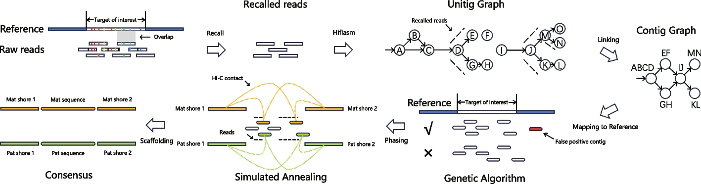
We use the term reference to indicate the high-quality genome assembly guiding TRFill and the term query to refer to the genome to assemble. We use the term target area of interest (TOI) to indicate the region that needs to be reassembled in the query genome. We use the term reference TOI to denote the corresponding region on the reference genome. The input to TRFill is (i) a reference genome, (ii) a chromosome-level query genome assembled using HiFi and Hi-C reads using a standard pipeline, e.g., hifiasm + 3D-DNA, (iii) HiFi and Hi-C reads for the query genome, and (iv) the starting and ending positions of TOI on the query genome. The output of TRFill is the reassembled sequence of the TOI in the query genome. TRFill operates in four phases: (1) recall all the HiFi reads that belong to the reads for the TOI; (2) assemble these recalled reads into contigs; (3) determine the contig positions and orientations using the reference; and (4) determine the phasing of the contigs. The TRFill pipeline is shown in Fig. 1 and Additional file 2: Fig. S1.

Read calling

TOIs are identified using the synteny between reference and query, which can be obtained using SyRI [39]. More specifically, the shortest continuous region on the reference that covers the TOI on the query is selected as the reference TOI. All HiFi reads are aligned to the reference TOI via winnomap2 [40] using the “-x map-pb” option. Any HiFi read which is partially aligned to the reference TOI is selected into a candidate set. Due to the expected difference between the reference and the query, it is not necessary to have the entire read aligned.

A hypothesis test is performed to remove as many false-positive reads from the candidate set as possible. The hypothesis is based on the presence of rare k-mers (in this study, we use 21-mers appearing less than 4 times in the whole reference genome). To obtain these rare k-mers, Jellyfish [41] is run to obtain the frequency of all the k-mers on the reference. For each read in the candidate set, we focus on its alignment with TOI on reference, and check if the rare k-mers in the aligned region in the reference also occur in the aligned region in the query. More formally, for an alignment \(A\) between the aligned region \(R\) on reference and the aligned region \(Q\) on read, let \(Y\) and \(X\) (\(X\le Y\)) be the number of rare k-mers in \(R\) and the number of rare k-mers in both \(R\) and \(Q\), respectively. We want to check how close are the value (\(x\)) of \(X\) to the value (\(y\)) of \(Y\). We assume \(X\) to be normally distributed, i.e., \(X\sim N(\mu ,^)\), where \(\mu\) is the number of rare k-mers appearing in both \(R\) and the corresponding region in the real query genome, and \(^\) is the sequencing error rate. Since the query genome and \(\mu\) are unknown, we further assume that \(\mu\) is a function of \(y\) if \(R\) and \(Q\) are homologous (i.e., \(R\) and \(Q\) are from the same tandem repeat in two different individuals, such as the centromeres of the same chromosome in two different genomes). Since \(\mu\) is always smaller than or equal to \(y\) by definition, we can assume that \(\mu =\delta y (0\le \delta <1)\). While parameter \(\delta\) is affected by many factors such as the difference in sequence composition between reference and query and the similarity in sequence composition within the TOI for both reference and query, for simplicity, we assume \(\delta\) to be constant. Since \(^\) is determined by the sequencing technology and only HiFi reads are used in this study, \(^\) is also assumed to be constant. With these assumptions in mind, the density function of \(X\) can be described as

$$_\left(x\right)=\frac^^}^}}}\sigma }.$$

Both \(\delta\) and \(^\) can have a drastic effect on the performance of TRFill. In this study, the values of \(\delta\) and \(^\) were estimated from the centromeric regions of Arabidopsis thaliana. A near-T2T-level assembly of the genome of Arabidopsis thaliana called ColCEN (accession Col-0) with almost complete centromeric regions was used as the reference. HiFi reads from the centromeric regions of accession Ler-0 [26] of Arabidopsis thaliana were aligned to the centromeric sequences of ColCEN. To obtain the HiFi reads from each centromere of Ler-0, we only kept the reads with high-quality alignments against the Ler-0 assembly (which contains almost complete centromeres). We denote by \(_\), \(1\le i\le N\) the set of alignments between HiFi reads from the centromeric regions of accession Ler-0 and the centromeric regions of ColCEN. Each \(_\) has associated variables \(_\), \(_\), \(_\), \(_\), \(_\), and \(_\) defined as we did above. The probabilistic density function of \(_\) can be described as

$$__}\left(_\right)=\frac^_- \delta _)}^}^}}}\sigma }.$$

By combining the probabilistic density functions of all \(_\) (\(1\le i\le N\)), the log likelihood function is obtained as

$$ln f\left(\delta , ^\right)=-\frac^\right)}-\frac_^_- \delta _\right)}^}^}.$$

By maximizing the log likelihood function, we can obtain a closed form for \(\delta\) and \(^\)

$$\delta =\frac_^__}_^_^}$$

Using these max likelihood estimates of \(\delta\) and \(^\), a two-sided test can be performed on each alignment \(A\) (with associated variables \(R\), \(Q\), \(X\), \(Y\), \(x\), and \(y\) defined above). Let \(_}\) be the value of a normal distribution at a certain significance level (e.g., \(\alpha =0.05\)). If \(x\) falls within \(\left[\delta y-_}\sigma , \delta y+_}\sigma \right]\), we recall the read. Otherwise, the read is a false positive and should be discarded. When a read has multiple alignments to the reference TOI, we perform a test for all alignments and recall the read as long as one alignment passes the test.

Contig assembly

After recalling HiFi reads, we assemble them into contigs. A unitig-level assembly graph is built from the reads with hifiasm. The default settings are used for a diploid genome, while option “-l0” is used for a haploid genome. Although hifiasm also provides a contig-level assembly graph, in some cases the contigs assembled directly from hifiasm have low completeness (see Additional file 2: Fig. S3). Instead, TRFill generates contigs from the unitig graph.

The HiFi reads are aligned to the unitig graph using winnowmap2 [35]. The number of supporting reads for each edge of the graph is counted. A modified breadth-first search (BFS) is used to traverse the unitig graph from zero-indegree nodes. A BFS-traversal graph, containing the same vertices as the unitig graph and all the edges in the unitig graph traversed by the modified BFS, is constructed, as follows. At each branching node v, rules (1–4) are followed. (1) We allow node v to be visited \(\lfloor (id+od)/2\rfloor\) times (instead of just once), where \(id\) and \(od\) are the in-degree and out-degree of \(v\), respectively; (2) for a successor node \(w\) of \(v\), if there exists a longer path from \(v\) to \(w\) in which \(o\) is the direct successor node of \(v\), \(o\) is chosen next rather than \(w\) (i.e., edge \(v\to w\) is seen as a transitive edge). Figure 1 shows a simple example with nodes \(A,B,C\) in unitig graph. Observe that there is a chance for \(w\) to be visited from \(v\), next time v is being visited. In case (2) does not apply, (3) among all the successors of \(v\) with enough supporting reads, the one with the largest number of supporting reads is chosen for visiting for this visit of \(v\) (see nodes \(M,O,N\) in unitig graph of Fig. 1 for an example). Similarly, there is a chance for other successors to be visited from \(v\), next time \(v\) is being visited. (4) If no successor of \(v\) has enough supporting reads, all successors of \(v\) are chosen for this visit of \(v\) (see \(D,E,G\) in unitig graph of Fig. 1 for an example). The BFS-traversal graph obtained by this modified BFS includes the order of the nodes visited and the corresponding timestamps. A node visited more than once will appear multiple times in the BFS-traversal graph with different order numbers.

A depth first search (DFS) is then used to traverse the BFS-traversal graph to generate contigs. As we did previously, each node is allowed to be visited \(\lfloor (id+od)/2\rfloor\) times, where \(id\) and \(od\) are the in-degree and out-degree. respectively. At each branching node \(v\), among all the successors of \(v\) such that their maximum number of visits has not been reached, we choose the one with the earliest timestamp in the BFS-traversal. We also mark where the graph needs to be cut after finishing the traversal to generate independent contigs. There is, however, a special situation when the graph can be solved. Additional file 2: Fig. S24A shows an example in which \(E\to A\to B\to C\to A\to D\) is a path that can generate a contig, although \(A\) is a branching node. To distinguish this case from other unsolvable situations, when a node is revisited and a loop is generated, we remove the cutting flag at that node. In the example, although \(A\) is marked to be cut after its first visit, the flag is removed at the second visit and we can generate the contig \(E\to A\to B\to C\to A\to D\). It is also possible to have an unsolvable branching node nested within a solvable loop. Additional file 2: Fig. S24B shows an example in which \(B\) is an unsolvable node and will be cut after the traversal while the other part of the loop is solvable, thus three contigs, namely \(E\to A\to B, C\to A\to D\), and \(F\), can be generated.

After the DFS traversal, the traversal graph is cut at the branching nodes determined by the following rules (1–3). Let \(v\) be a branching node. (1) If \(v\) has one predecessors and multiple successors, the outgoing edges of \(v\) are cut and the incoming edge is kept. (2) If \(v\) has multiple predecessors and one successor, the incoming edges of \(v\) are cut and the outgoing edge is kept. (3) If \(v\) has multiple predecessors and multiple successors, all the incoming edges and outgoing edges of \(v\) are cut.

Determining the position and orientation of contigs

After obtaining the contigs, TRFill determines the contig positions and orientations relative to the reference. First, the contigs are mapped to the reference TOI with winnowmap2 and filtered out if they have a poor alignment. A contig is discarded if either (1) its alignment to the reference TOI is shorter than 10% of its lengths, or (2) the total length its alignment to the reference TOI is less than twice the total length its alignments to other regions on reference genome.

TRFill then determines the positions and orientations of the remaining contigs according to their alignments to the reference. This step is challenging due to the fragmented alignments caused by the differences between the reference genome and the query genome and the multiple alignments due to the highly repetitive sequences. We framed this problem in a combinatorial optimization model. Let us assume that a contig is mapped to the reference TOI along a set of fragmented alignments. For each alignment, we define an aligned pair defined by (reference region, contig region) as an element. By sorting the elements for a given contig by their starting positions on the contig, we obtain a sorted sequence \(_[1\dots N][1\dots N]\) of elements for the contig. On reference side, we check all subregions of the TOI with a length equal to the contig length starting from the element aligned to \(_[1]\). For each of these subregions, a sequence \(_[1\dots M]\) of elements on the reference side is obtained. The alignment score between the contig and a subregion is the length of the longest matching subsequence (see Definition 1 below) between \(_\) and \(_\) where the “matching” in LMS represents the “alignment” between elements.

Definition 1 (longest matching subsequence)

Input: a sequence \(A[1\dots N]\) of elements, a sequence \(B[1\dots M]\) of elements, and a matching function \(f\) in which \(f(x, y)=True\) if element \(x\) in \(A\) matches element \(y\) in \(B\). Output: a subsequence \(A\) of \(A\) and a subsequence \(B\) of \(B\) such that (i) \(|A|\) = \(|B|\) and (ii) for any position \(k (1\le k\le |A|)\), \(f(x, y)=True\) for element \(x\) in \(A\) element \(y\) in \(B\) at the position kth position.

Since LMS is a variant of the longest common subsequence problem, LMS can also be solved optimally in \(O(NM)\) time. This complexity, however, might be too high for some contig with very fragmented alignments. To speed up this step, we generate an approximate solution of LMS by solving the longest increasing subsequence problem (LIS) [42]. Given the sequence \(_\) of elements on the reference, a corresponding coordinate sequence \(L[1\dots M]\) of same length is built according to the sequence \(_\) of elements on the contig. For any \(j (1\le j\le M)\), \(L[j]=i\) if \(_[j]\) is aligned to \(_[i]\). A longest increasing subsequence \(LL[1\dots P]\) satisfying criteria 1 and 2 below is obtained with a binary search algorithm [43] in \(O(N+M log M)\) time. The criteria are the following. (1) \(LL\) is a subsequence of \(L\); (2) for any choice of \(p, q (1\le p<q\le P), LL[p]\le LL[q]\); (3) there exists no other subsequence of \(L\) satisfying (1) and (2) with length longer than the length of \(LL\). The length of the longest increasing subsequence is used as the alignment score between the contig and the subregion of the reference TOI. For each contig, we select as candidates at most seven subregions with the highest alignment score.

TRFill uses a genetic algorithm to select the optimal subset of these contigs and determine their positions. Each contig, each alignment position, and each possible combination of candidate alignment positions of contigs represent a locus, an allele, and an individual, respectively, in the terminology of genetic algorithms. We simulate the evolution process by carrying out switching operations (i.e., switch alignment position of one contig between two individuals), variation operations (i.e., delete or insert one contig from or to individual), and natural selection operations (select individuals with a probability proportional to the fitness score). The objective is to obtain individuals that maximize the objective function (also called the adaptivity of individuals). The objective function has two components, one related to the coverage and one related to the distance. The coverage component aims to ensure that the contigs collectively cover the entirety of the reference TOI exactly \(T\) times, where \(T\) represents the ploidy of the query genome (e.g., \(T=2\) for a diploid genome). The distance component aims to maximize the distance between contigs to reduce the extent of overlap between them. Observe that these two objectives work against each other: covering the reference more extensively tends to bring contigs closer together.

Formally, let \(_\) be the total length of the subregions of the reference TOI with a coverage of \(t\), and \(_ (i,j\in \left[1, C\right])\) be the distance between alignment midpoints of contig \(i\) and contig \(j\) on the reference TOI where \(C\) represents the total number of contigs. The objective functions for haploid and diploid genomes are as follows.

$$_=2\left(_-_-_\right)+_-2.5_+\frac_^_^_$$

$$_=2\left(_-_\right)-_-2.5_+\frac_^_^_$$

where \(_\) represents the total length of a special type of subregions with coverage 0 in which the contigs aligned to its left and right belong to the same connected component in contig-level assembly graph. Since these types of subregions should not exist, we give them a higher penalty. \(_\) represents the total length of other subregions with coverage 0.

The genetic algorithm proceeds in the following steps:

(1)

Initialization: randomly generate 500 individuals

(2)

Termination: calculate the adaptivity (objective function) for each individual; the algorithm terminates if either the 10 individuals with the highest adaptivity have the same adaptivity or if the algorithm has been executed for a maximum number of iterations (200)

(3)

Natural selection: select 60 individuals from the pool of 500 according to their adaptivity (individuals with higher adaptivity are selected with higher probability)

(4)

Switching: select two individuals from the pool of 60 at random, and use them to generate two offspring individuals by randomly switching their alleles (the alignment position of the contig) at one same locus (contig)

(5)

Variation: for each of the offspring individual, add a mutation with a probability of 0.05 by either deleting one locus (contig) and its corresponding allele (the alignment position of the contig) or adding one locus (contig) and one of its allele (one of the candidate alignment positions of the contig)

(6)

Repeat (4–5) until 300 offspring individuals are generated, and then go to (2) for the next iteration

After the termination, TRFill selects the subset of contigs and the combination of candidate alignment positions of contigs in the subset from the individual with the highest adaptivity.

Phasing

Once TRFill has determined the positions of contigs on the reference, the final step is to generate the sequence for the query TOI. For a haploid genome, the contigs are directly connected into scaffolds by adding a fixed number of “N”s. For a diploid genome, the phasing process uses HiFi and Hi-C reads (and the homology between the contigs). Since HiFi and Hi-C provide linkage information with different resolutions, TRFill uses them in different ways. HiFi reads are used to link the contigs belonging to the same haplotypes, while Hi-C reads are used to link the contigs and the genomic regions flanking the TOI in the query genome (hereafter called shores). To obtain allele-specific Hi-C information, we only consider Hi-C pairs with both ends on unique k-mers (i.e., k-mers appearing only once on contigs and shores, k = 31). Hi-C reads are positioned on the contigs and the shores according to their unique k-mers rather than based on sequence alignment. HiFi signals are instead obtained by aligning the HiFi reads to the contigs using winnowmap2, rather than using unique k-mers. We expect that the number of HiFi reads linking contigs on the same haplotypes are much higher than the ones incorrectly linking contigs on different haplotypes. We also expect that contigs with higher homology should belong to the same haplotype with lower probability. The homology coefficient between each pair of contigs is computed from the number of shared k-mers. If the set of all k-mer in contig \(i\) is \(_\), and the homology coefficient between contig \(i\) and contig \(j\) is \(_=\frac_ \wedge _\right|}_\right|,\left|_\right|)}\). The global homology coefficient \(h\) is the average of all non-zero values of \(_\).

Given the HiFi and Hi-C signals and the homology coefficients, we set up a combinatorial optimization framework to solve the phasing problem. Let \(_\) be the length of sequence \(i\) (contig or shore); \(\underline\) be the average value of the homology coefficients for all pairs of contigs; \(_\), \(_\), \(_\), \(_\) be the sets of shores and contigs assigned to the maternal and paternal haplotypes (collapsed contigs will appear in both \(_\) and \(_\)); \(_, _, _, _\) be the number of Hi-C signals, the number of HiFi signals, the distance, the homology coefficient between sequence \(i\) and sequence \(j\), respectively. The objective function is as follows.

$$f=C_1\left(\sum\nolimits_i^_}\sum\nolimits_j^_}\frac_}}+\sum\nolimits_i^_}\sum\nolimits_j^_}\frac_}}\right)+C_2\left(\sum\nolimits_i^_}\sum\nolimits_^_}\frac\right)HIFI}_}+\sum\nolimits_i^_}\sum\nolimits_^_}\frac\right)HIFI}_}\right)-_\frac_^_}_-_^_}_|}_}$$

The objective function has three components, weighted by parameters C1, C2, and C3. The first component rewards Hi-C signals linking the shores and contigs on the same haplotypes. The second component captures two distinct situations. When \(\underline-_\) is positive (i.e., there is low homology between contig \(i\) and \(j\)), then \(_\) contributes positively to the objective function thus rewarding HiFi signals connecting the contigs in the same haplotypes. A higher value of \(_\) leads to a lower \(\underline-_\) which results in a lower score of objective function, representing the negative effect on the homology. When \(\underline-_\) is negative (i.e., there is high homology between contig \(i\) and \(j\)), \(_\) contributes negatively to the objective function. The structure of the second component deals with homologous contigs from different haplotypes which may have HiFi reads connecting them due to the high sequence similarity of the underlying repetitive sequence. The third component penalizes the length difference between the assembled maternal and paternal TOI sequences.

To maximize this complex objective function within an acceptable time, TRFill uses an algorithm inspired by simulated annealing. Each contig can be in one of four states: 0 (discarded), 1 (maternal), 2 (paternal), or 3 (collapsed). The algorithm proceeds as follows.

(1)

Initialization: randomly set the state of each contig; set the global maximum to a very large negative number

(2)

Termination: calculate the value of objective function; if this step has been executed for 1000 times, exit

(3)

Change the state of a random contig if it improves the value of objective function

(4)

Repeat step (3) until the value of objective function remains unchanged for 100 consecutive iterations and thus a local maximum is obtained; if the local maximum is higher than the current global maximum, set it as the new global maximum

(5)

Randomly change the states of a fraction of the contigs (50%) to prevent the algorithm from getting stuck from on maxima. Go to step (2)

The final assembly may include some portions of the flanking sequences (shores) because TRFill might assemble reads that overlap the shores. To correct for this issue, TRFill trims these sequences based on an alignment of the final scaffolds against the shores. Finally, the repetitive regions (TOIs) in each haplotype are replaced by the corresponding trimmed scaffolds.

Evaluation on human centromeric alpha satellite arrays

TRFill was tested on a diploid human genome HG002 (NA24385). The HiFi data (~ 36 × coverage) and Hi-C data (~ 69 × coverage) for this sample was generated by the Human Pangenome Reference Consortium (HPRC) [28]. The corresponding haplotype-resolved high-quality assembly was used as the “ground truth.”

First, we generated a chromosome-level diploid assembly of HG002 to provide as input to TRFill. We used hifiasm (v0.19.5-r587) on HiFi and Hi-C data with default parameters to produce a haplotype-resolved assembly. We used 3D-DNA (branch 201,008) with the “-r 0” option for scaffolding, then manual curation based on Hi-C heap map via Juicebox [44].

The human haploid T2T genome (CHM13 v2.0) was used to guide our assembly of HG002. The positions of the TOIs on HG002 were lifted from the positions of centromere alpha satellite sequences on CHM13, as follows. First, the position of centromere alpha satellite sequence on each chromosome on CHM13 was determined from the downloaded annotations and the results from Tandem Repeat Finder (TRF, v4.09.1) [45]. When a chromosome of CHM13 contained multiple pieces of the alpha satellite sequences, only the longest continuous alpha satellite sequence was considered. SyRI (v1.6) with default parameters was used to build the synteny between CHM13 and the two haplotypes of HG002. The regions of HG002 that aligned to the selected alpha satellite sequences on CHM13 were chosen as the TOI. If the TOI were partially assembled in the chromosome-level assembly of HG002, we removed them and replaced them with a continuous gap for each TOI. We used TRFill, LR_Gapcloser, and SAMBA (v4.1.0) to reassemble the TOIs. TRFill used the CHM13 assembly as reference.

Several criteria were used to comparatively evaluate the quality of the assemblies TRFill, LR_Gapcloser, and SAMBA in terms of contiguity, completeness, and accuracy. First, the TOI assemblies were aligned to the ground truth using winnowmap2. Any region corresponding to a continuous alignment was considered a correct genomic region. We defined completeness as the ratio between the total length of the correct regions and the total length of the ground truth. We defined correctness as the ratio between the total length of correct regions and the total length of assembly. We defined the LIS score as the ratio between (i) the length of the longest increasing subsequence between the unique k-mers in the ground truth assembly and the TOI assembly and (ii) the number of unique k-mers in the TOI assembly (see section Determining Positions and Orientations of Contigs in Methods for the generation of LIS).

The strictly-improved and loosely-improved criteria are defined based on the R_AQI and S_AQI scores generated by CRAQ, as well as the HiFi read coverages for both the TRFill and the original assemblies. The R_AQI and S_AQI scores were obtained by running CRAQ with either the TRFill or original assembly, along with the whole-genome HiFi reads as input, using the “-x map-hifi” parameter. HiFi read coverage was calculated by aligning the whole-genome HiFi reads to the respective assemblies using winnowmap2 with default settings.

First, let R_AQI_ori, S_AQI_ori, R_AQI_new, S_AQI_new, cov_ori, and cov_new represent the R_AQI, S_AQI, and HiFi read coverage for the original and TRFill assemblies, respectively. Let cov_whole denote the average genome-wide HiFi read coverage. A gap is considered strictly improved if R_AQI_new > R_AQI_ori × 1.1. A gap is considered loosely improved if R_AQI_new > R_AQI_ori, or if the conditions (1–3) are met. Condition (1) R_AQI_new > R_AQI_ori/1.6; condition (2) S_AQI_new > S_AQI_ori; condition (3) |cov_whole – cov_new| <|cov_whole – cov_ori|.

Evaluation on tomato subtelomeric tandem repeats

For the analysis of tomato subtelomeric tandem repeats, we built a comprehensive dataset for Heinz1706, TS2, and TS281 using publicly available data and our own sequencing. We generated ONT UL sequencing data for all three, and Illumina Hi-C sequencing for TS2 and TS281. We were able to obtain Hi-C data for Heinz1706 and HiFi data for all three on public repositories. Our sequencing sample was collected from young leaves of a tomato plant at the Agricultural Genomics Institute at Shenzhen, Chinese Academy of Agricultural Sciences (Guangdong province, China). For the ONT UL sequencing, high-molecular-weight genomic DNA selected with SageHLS HMW library system (Sage Science). DNA was processed with the Ligation sequencing 1D Kit. The library was constructed using the approach described in Wang et al. and sequenced on the Nanopore PromethION platform at the Genome Center of Grandomics (Wuhan, China). For the Hi-C sequencing, the library was constructed and sequenced using the approach described in Rao et al. and sequenced using the Illumina NovaSeqX-plus platform at the Genome Center of Grandomics (Wuhan, China). The restriction enzyme used for Hi-C library construction is DpnII from NEB.

To build the reference genome (Heinz1706) and two ground truth genomes (TS2 and TS281), we assembled them individually de novo. We used hifiasm (v0.19.5-r587) with the “-ul” and “-l0” options to generate contigs based on HiFi and ONT UL reads. We used 3D-DNA (branch 201,008) with the “-r 0” option for scaffolding using Hi-C reads.

In the experiments for the haploid genome, the subtelomeric tandem repetitive regions of TS2 and TS281 were the TOIs that were reassembled with TRFill (guided by the Heinz1706 reference genome). The chromosome-level assembly of TS2 and TS281 was obtained from SolOmics (http://solomics.agis.org.cn/tomato/ftp). These assemblies were generated exclusively from HiFi data. TRFill was used to assemble the TOIs.

In the experiments on the diploid genomes, the TS2 and TS281 haplotype assemblies were merged to produce a pseudo-diploid genome. The HiFi and Hi-C data for both TS2 and TS281 were merged to simulate data for the pseudo-diploid genome. Since the merged Hi-C data lacked the inter-chromosome read pairs between the maternal and paternal chromosomes, additional Hi-C read pairs were added into the Hi-C data set. We used sim3C [46] with default parameters to generate synthetic Hi-C reads at 130 × sequencing depth using the ground truth genome as the reference. Synthetic read pairs between maternal and paternal chromosomes were selected and added to the real Hi-C reads.

The chromosome-level assembly of the diploid genome was generated using hifiasm (v0.19.5-r587) using HiFi and Hi-C data. Scaffolding was carried out with 3D-DNA using Hi-C data.

The subtelomeric tandem repeats (query TOI regions) were identified using the reference genome. TRF (v4.09.1) was used to detect repetitive patterns within the reference sequences. We identified regions located at the edge of each chromosome that harbor 181 bp-long monomers. Not every chromosome had both pairs of subtelomeric repeats, and some chromosomes contained the 181 bp monomers not at the chromosome ends. The TOI regions on the query were identified using the synteny between the reference and the query determined by SyRI (v1.6).

Population-level analysis of tomato subtelomeric tandem repeat units

Chromosome-level assemblies for 29 tomato genomes were downloaded from SolOmics (http://solomics.agis.org.cn/tomato/ftp). The subtelomeric tandem repetitive regions were assembled by TRFill with the same pipeline as the validation experiments of the haploid tomato genome using Heinz1706 as the reference. For each subtelomeric tandem repeat, if the TRFill assembly was longer than the original one, we kept the TRFill assembly (the original sequence was kept otherwise).

The population-level analysis used the Tandem Repeat Annotation and Structural Hierarchy (TRASH) [47]. Both monomer mode and HOR mode were used in TRASH to detect the monomers and HORs from the tandem repeat sequences, providing coordinates, orientation, and length of each repeat unit.

For the analysis of monomers and HORs, the 181 bp consensus sequence of the monomer was built by carrying out a multiple sequence alignment. A consensus monomer sequence for each subtelomere was built according to sequence alignment of all the monomers in each subtelomere (using mafft2 [48]). The global consensus sequence was generated by a multiple sequence alignment (again, using mafft2) of all subtelomere-level consensus sequences.

To analyze the sequence similarity of monomers, we carried out comparisons between (1) the intra-genome monomers and inter-genome monomers, (2) intra-chromosome and inter-chromosome monomers on the same genomes, and (3) intra-subtelomere and inter-subtelomere monomers on the same chromosomes. For each of these comparisons, a series of experiments were carried out, each of which computed the pairwise similarity between a randomly selected pair of monomers. The pairwise similarity was defined as the ratio between the number of common monomers in the two sets and the total number of monomers in both sets. For the random experiments (1) and (2), each of the two sets contained all monomers from a randomly selected subtelomere. For the random experiments in (3), each of the two sets contained one tenth of the monomers in a randomly selected subtelomere, and the two sets did not contain the same monomers for intra-experiments. The similarity calculations between all pairs of subtelomeres was defined in the same way.