Data

The data of two antidepressant RCTs were used as cases-study. The first one, study 810, was a randomized, double-blind, parallel-group, placebo-controlled study evaluating efficacy and safety of paroxetine CR 12.5 mg/day (N = 156), paroxetine CR 25 mg/day (N = 154) versus placebo (N = 149) in patients with MDD and a mean age (± StdErr) of 39 (± 0.5) years. The primary efficacy endpoint was the change from baseline at week 8 in the 17-item Hamilton Rating Scale for Depression (HAMD-17) [23]. The second one, study 874, was a randomized, double-blind, parallel-group, placebo-controlled fixed-dose study evaluating the effect of of paroxetine CR 12.5 mg/day (N = 161), paroxetine CR 25 mg/day (N = 173) versus placebo (N = 178) in patients with MDD and a mean age (± StdErr) of 67 (± 0.3) years. The primary efficacy endpoint was the change from baseline at week 8 in the HAMD-17 scale [24].

Clinically relevant non-treatment specific response

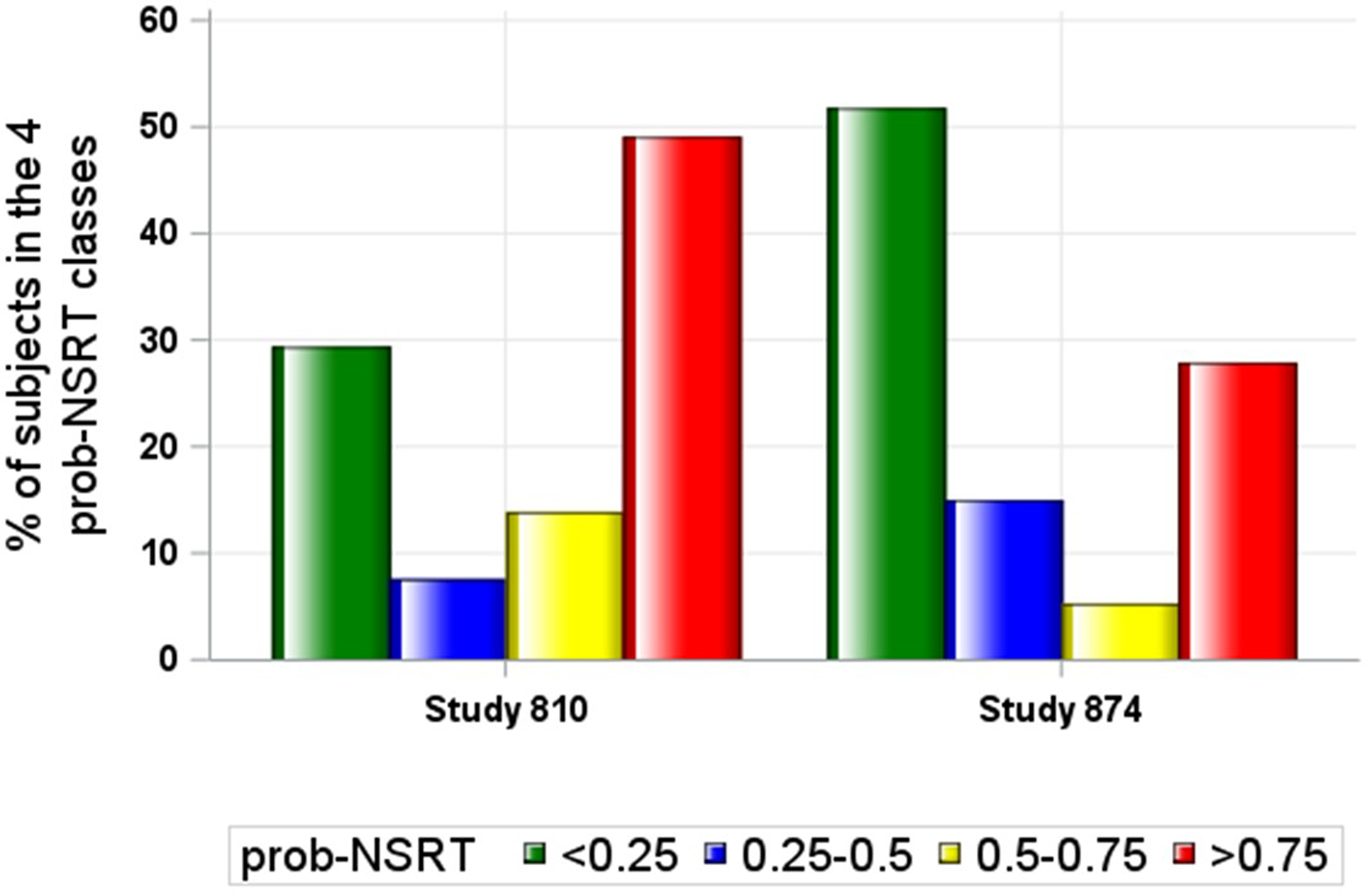
The clinical response was assessed using the longitudinal change of HAMD-17 total score [25]. The clinically relevant non-specific response was defined using the score of the Clinician Global Impression-Improvement (CGI-I) scale as this score represents a patient-independent assessment done by the clinician on the patient’s global disease severity prior to and after initiating the treatment. A CGI-I between minimally improved (= 3) and much improved (= 2) was considered as an indicator of a clinically relevant response. This CGI-I score was associated to a percent reduction from baseline at week 8 in the HAMD-17 total score of 41% using the equipercentile linking method [26,27,28]. A binary score (0 or 1) was then associated to each subject in the placebo arm as an indicator of the absence or presence of a clinically relevant signal of response at EOS when the change from baseline of HAMD-17 total score was greater than 41%.

AI model development

Six machine learning methodologies (gradient boosting machine, lasso regression, logistic regression, support vector machines, k-nearest neighbors, and random forests) were compared to the multilayer perceptrons artificial neural network (ANN) methodology for predicting the probability of individual non-specific treatment response. ANN achieved the highest overall accuracy among all methods tested. For this reason, the ANN method was retained as the reference methodology for estimating the individual prob-NSRT.

The individual HAMD-17 items collected at two pre-randomization time points (i.e., at screening and baseline) were used to predict the prob-NSRT at EOS using an artificial neural network (ANN) methodology [29]. The implementation of an ANN model requires the definition of two hyperparameters that control the topology of the network: the number of hidden layers and the number of nodes in each hidden layer. A preliminary grid search analysis was conducted to identify these parameters using optimality criteria. These criteria were based on the best predictive performance of the ANN model defined by:

The ROC AUC: Area under the Receiver Operating Characteristic curves with the 95% confidence intervals. The larger the ROC AUC the better the predictive performance of the model. The area of 1.0 is associated with the ideal predictor because it achieves both 100% sensitivity and 100% specificity. The area of 0.5 is associated with a poor predictor with 50% sensitivity and 50% specificity. A reliable and informative predictor should have an area statistically larger than 0.5.

The Sensitivity or Recall: the ratio of true positives to total positives in the data.

The Specificity: the ratio of true negatives to total negatives in the data.

The Accuracy: the number of correct predictions as a fraction of total predictions.

The Precision: the fraction of correct positive predictions.

The ANN analysis was conducted using the ‘neuralnet’ library in R [30]. A formal procedure for the ANN model development and validation was applied. According to this procedure, the available data were split into three datasets:

1.

The training set, applied for the ANN model development (in our case this dataset included 75% of the data in the placebo arm randomly selected).

2.

The validation set used to assess the model performances in data not used for model development (in our case this dataset included the 25% data in the placebo arm not used for model development).

3.

The working dataset, with the full data set including all the subject data in the 3-arms together with the individual estimate of the propensity probability estimated using the ANN model applied to the pre-randomization data of each subject in each treatment arm.

The ANN model, developed and validated using placebo data, was applied to the individual HAMD-17 item changes from screening to baseline of each subject in the three arms to estimate the individual prob-NSRT.

Propensity score analysis

Different propensity score methods have been proposed for removing the effects of confounders when estimating TE. Among these methods, we retained the inverse propensity score weighting (PSW), and the covariate adjustment using the propensity score [31].

The PSW methodology was finally retained as the main objective of the analysis was to assess the mean TE in a given population accounting for the individual estimate of the treatment-specific and non-specific responses. The inverse of the individual prob-NSRT was used as an estimate of the ‘true’ contribution of each subject enrolled in the trial for assessing TE. Differently from this approach, the covariate adjustment would have been more appropriate for explaining and controlling the inter-individual variability of the model parameters rather than for providing an adjusted mean TE estimate.

Inverse probability of treatment weighting analysis

The analysis was conducted in two stages. In stage 1, the data of the study 810 and 874 were independently analyzed for estimating the individual prob-NSRT using the ANN models. In stage 2, the data of the two studies were jointly analyzed using a PSW methodology to estimate the TR and the TE using a non-linear mixed effect modeling approach.

The analysis was conducted using a 6-step approach:

Step 1: The pre-randomization (i.e., screening and baseline) and end of study data (EOS) (i.e., visit on week 8) in subjects randomized to placebo were selected.

Step 2: A predictive model was developed to estimate the probability to be placebo responder (prob-NSRT) after 8 weeks of treatment using the ANN model and pre-randomization data.

Step 3: The model developed in step 2 was validated by comparing the model predicted probability to the observed placebo response.

Step 4: The ANN model developed in step 2 was used to predict the individual prob-PE using the pre-randomization data of all subjects randomized in the study.

Step 5: The individual prob-NSRTj value was estimated by applying the ANN model to the pre-randomization data of each subject enrolled in the trials.

Step 6: The individual prob-NSRT value (prob-NSRTj) was included as individual weight in non-linear mixed effect (NLMMRM) model used for analyzing the longitudinal HAMD-17 total scores and for estimating the treatment effect (TE): higher is prob-NSRTj), lower will be the contribution of the jth subject to the TE estimation.

Longitudinal model

Two parallel independent analyses were conducted. The first one identified as ‘reference’ analysis was based on the conventional non-weighted non-linear regression analysis and the second one, identified as ‘propensity’, was based on the PSW methodology. The ability of the two analyses to assess the TE accounting or not for the presence of non-specific treatment response was assessed by comparing the results of the two analyses.

A model describing the longitudinal time-course of the HAMD-17 total scores was used to jointly describe the pooled dataset of the 810 and 874 studies. This model data were described by the Weibull function:

$$P\:\left( t \right) = A^b}}} + }t + eps$$

(1)

were P(t) is the HAMD-17 total clinical score at time t, A is the baseline HAMD-17 total score, td is the time corresponding to a 63.2% reduction of HAMD-17 from baseline, b is the rate of change in response, hrec is the recovery rate and eps is the residual error. This model was previously applied to describe the HAMD-17 longitudinal response in different RCTs conducted in MDD populations [17, 21].

As the primary endpoint of the two selected RCTs was the change from baseline of the total HAMD-17 score at week 8 (t = 8), the model was re-parameterized in order to include a parameter defining the HAMD-17 total score at week 8 (F8) and the change from baseline of the HAMD-17 total score (TR) at week 8:

$$F8 = A\:^b}}} + }8$$

(2)

where

The change from baseline of the HAMD-17 total score (TR) at week 8 was estimated as:

The proposed model included three fixed-effect parameters: td, b, and F8. The value of A was fixed to the individual observed HAMD-17 total score at baseline.

The inter-individual variability (IIV) model was assumed to be log-normally distributed. The relationship between a parameter P(td, b, and F8) and its variance was therefore expressed as:

Where Pj is the value of parameter for the jth individual, PTV is the typical value of P for the population, and \(\eta P\) denotes the difference between Pj and PTV, normally distributed with a mean zero and variance\(\:\omega \). The residual error model (epsj) for the ‘reference’ analysis was defined as epsj = ε, where ε is normally distributed with mean 0 and variance s2.

The individual propensity (prob-NSRTj) for a non-treatment specific response was implemented in the longitudinal model as a subject specific weight in the residual error model (epsj). This model was defined as the ratio between components ε and Wj:

$$ep = \varepsilon /Wj$$

(6)

where ε is normally distributed with mean 0 and variance s2 and Wj is the individual weighting factor defined as:

$$ = 1} - \left( } \right)$$

(7)

According to this model, a weight Wj was associated to each individual data: the subjects with lower Wj (reflecting higher uncertainty in the measurements for this individual) were considered as less informative and contributed less to the estimation of the model parameters and to the assessment of TE.

The parameters were estimated using the NONMEM software (version 7.5.1) using the stochastic approximation expectation-maximization (SAEM) with the interaction computational algorithm. The − 2 loglikelihood (–2LL) value at the final model parameter estimates was calculated using the importance sampling approach (IMP). Model selection was based on likelihood-ratio test. An alternative nested model was considered statistically significant if it decreases − 2LL more than 3.84 (P < 0.05 with 1 degree of freedom).

Covariate analysis

The only prospectively identified covariates were dose and age. The impact of dose and age were evaluated on each of the three parameters of the longitudinal model: td, b, and F8. A dose = 0 was associated to the data in the placebo arm. The stepwise covariate model building procedure (SCM) was used to identify the relevant covariates [32] with a significance alpha level of 0.05 and of 0.01 for forward and backward selections, respectively.

Longitudinal model evaluation

The final ‘reference’ and ‘propensity’ models evaluation was accomplished by assessing the models for the goodness-of-fit plot, which included individual and population-predicted versus observed HAMD-17 scores, conditional weighted residual versus time and population-predicted HAMD-17 scores. The reliability and stability of the final longitudinal models were further assessed by a nonparametric bootstrap resampling method. Two thousand bootstrap datasets were generated by randomly sampling with replacements from the original dataset to form new datasets containing the same number of patients as the original dataset. The median parameter values and nonparametric 95% confidence intervals (CI) were derived from the NONMEM fit based on the 200 bootstraps dataset and compared with the final parameter estimates [13]. Furthermore, prediction-corrected visual predictive checks (pcVPCs) were performed to explore the predictive capability of the final longitudinal models [14]. The final model parameter estimates and the demographics information of subjects were used for simulating 200 new virtual clinical trials. The median and the 95% prediction interval simulated plasma concentration was plotted and compared with the observed data.