1 Introduction

Gait refers to the distinctive walking pattern unique to each individual (Saleh and Hamoud, 2021). It involves a cyclic sequence of movements in both lower limbs (Jing et al., 2019), providing valuable information about individuals' physical and physiological attributes, including weight, gender, health, and age (Wang and Zhang, 2020; Sadeghzadehyadi et al., 2021).

Gait analysis holds immense importance across various domains, such as healthcare, sport, biometrics, and human–robot interaction. It serves as a rich source of information, adding to the understanding and assessment of various conditions, including neurodegenerative disorders like Parkinson's disease (PD) (Alotaibi and Mahmood, 2015; Yuqi et al., 2019; Chaabane et al., 2023).

Previous studies (Castro et al., 2017; Huang et al., 2021; Wang and Yan, 2021; Erdaş et al., 2022; Vidya and Sasikumar, 2022) have explored gait analysis in the context of PD, aiming to diagnose the condition and track disease progression (Yuan and Zhang, 2018; Zhang S. et al., 2019; Mogan et al., 2023). However, these analyses often rely on clinical evaluation and subjective surveys, resulting in semi-subjective assessments (Wu et al., 2016; Arshad et al., 2021; Khan et al., 2023). Additionally, gait alterations under cognitive load known as “dual tasks” have been investigated, revealing variations influenced by factors such as environmental conditions and emotional states (Delgado-Escaño et al., 2018; Alharthi et al., 2019; Castro et al., 2020; Slijepcvic et al., 2021).

The existing gait analysis in literature faces limitations, particularly in accurately representing the non-linearity and non-stationary of gait cycle (Whittle, 2023). Traditional methods, such as visual observation and harmonic analysis, may fall short of capturing the intricate dynamics of gait (Goodfellow et al., 2016). To address these limitations, this study incorporates explainable artificial intelligence (XAI) techniques. XAI, including layerwise relevance propagation (LRP), enhances the transparency of deep learning models, adding to the interpretation of predictions. We selected LRP over other XAI methods, such as SHAP (SHapley Additive ExPlanations) (Ribeiro et al., 2016), Gradient-weighted Class Activation Mapping (Grad-CAM) (Selvaraju et al., 2017), and Local Interpretable Model-agnostic Explanations (LIME) (Lundberg and Lee, 2017). As noted by Adebayo et al. (2018), not all proposed XAI methods are robust, and the validity of their explanations should be critically assessed.

In this paper, we contribute a comprehensive approach to gait analysis by leveraging sensor fusion, deep convolutional neural networks (CNN), and XAI techniques, specifically LRP. The utilization of CNNs facilitates automatic feature extraction from raw sensor data, while the incorporation of LRP enhances interpretability. This novel combination adds significant value to the fields by providing insights that inform not only gait analysis but also sensor design and data processing for improved healthcare applications.

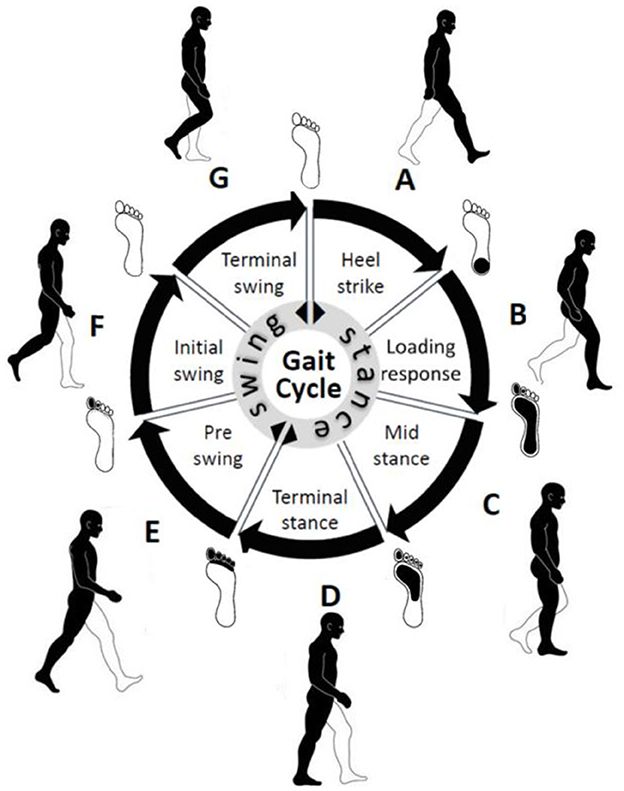
2 Background 2.1 Related studies

Gait, the intricate walking pattern unique to each individual, has captivated humans (Wang and Zhang, 2020). Figuratively, the gait cycle, as depicted in Figure 1, encapsulates the rhythmic sequence of movement in the lower limb during walking. Early civilizations recognized the distinctiveness of gait as a personal identifier, and over time, methodologies for studying gait have evolved from rudimentary visual observation to sophisticated techniques (Yuqi et al., 2019).

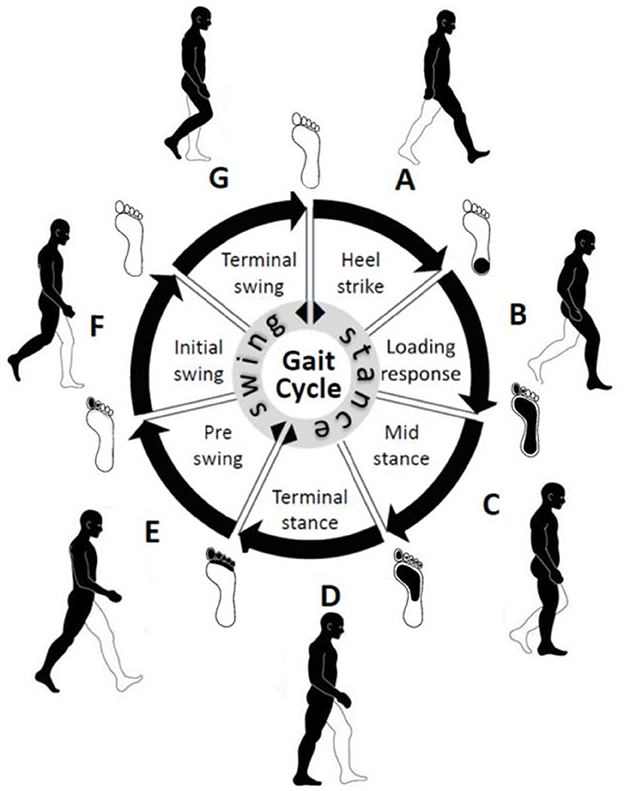
Figure 1. Important gait events and intervals in a normal gait cycle. In the center, the stance phase represents 60% of the gait cycle and the swing phase represents 40% of the gait cycle.

In ancient times, the recognition of individuals based on their gait laid the foundation of contemporary studies (Saleh and Hamoud, 2021). Recent advancements, such as the integration of CNN, have enabled person recognition through intricate gait models (Jing et al., 2019). These efforts underscore the enduring importance of gait analysis, with applications ranging from healthcare to biometrics (Alotaibi and Mahmood, 2015).

The landscape of gait analysis has witnessed a notable surge in recent literature, with cutting-edge technologies at the forefront. For instance, a fusion network incorporating long short-term memory (LSTM) and CNNs demonstrated heightened accuracy in abnormal gait recognition (Sadeghzadehyadi et al., 2021). Another study applied a CNN-LSTM network to decipher spatiotemporal patterns of gait anomalies (Wang and Zhang, 2020), highlighting a continuous evolution of gait analysis methodologies.

Gait biometrics has emerged as a focal point, with studies exploring joint CNN-based methods (Chaabane et al., 2023). Moreover, predicting the severity of neurodegenerative diseases using CNNs showcased promising outcomes (Yuqi et al., 2019). Lightweight attention-based CNN models efficiently recognized gait patterns using wearable sensors, pushing the boundaries of gait analysis capabilities (Alotaibi and Mahmood, 2015). These contemporary studies collectively underscore the growing importance of leveraging advanced technologies for accurate and nuanced gait analysis.

Recent gait recognition literature has focused on solving view- and clothing-invariant problems using advanced machine learning methods like generative adversarial networks (GANs). Zhang P. et al. (2019) designed a view transformation GAN (VT-GAN) with a generator, discriminator, and similarity preserver, achieving competitive results on the CASIA-B dataset. Babaee et al. (2019) used GANs to reconstruct complete gait energy images (GEIs) from incomplete ones, showing effectiveness on the OU-ISIR dataset. Chen et al. (2021) proposed Multi-View Gait GAN (MvGGAN) for cross-view gait recognition, demonstrating improved performance on CASIA-B and OUMVLP datasets. Recent study on wearable and floor sensors has focused on medical applications, such as analyzing the impact of muscle fatigue on gait (Balakrishnan et al., 2020), health monitoring (Muheidat and Tawalbeh, 2020), and age-related differences (Costilla-Reyes et al., 2021). Turner and Hayes (2019) proposed using an LSTM network to classify pressure sensor signals from shoes, aiming to diagnose gait abnormalities. Tran et al. (2021) developed multi-model LSTM and CNN to classify IMU spatiotemporal signals, outperforming previous results on the whuGAIT (Zou et al., 2020) and OU-ISIR (Ngo et al., 2014) datasets.

In the field of gait analysis, the integration of explainable artificial intelligence (XAI) represents a pioneering approach. XAI techniques, exemplified by methods such as layerwise relevance propagation (LRP), address the opacity challenge inherent in deep learning models (Erdaş et al., 2022). LRP has shown success in image classification (Samek et al., 2017a; Jolly et al., 2018) and gait-based subject identification (Horst et al., 2019) when combined with CNNs. Our study stands as a beacon of innovation, presenting a comprehensive approach that seamlessly integrates sensor fusion, CNN, and XAI techniques for gait analysis (Khan et al., 2023).

While existing studies have explored gait analysis through the lens of deep learning models, our distinctive contribution lies in the transparent interpretation facilitated by XAI. Building on recent advancements, we propose using LRP to enhance the interpretability of CNN predictions (Castro et al., 2020). This not only adds intrinsic value to gait analysis but also provides profound insights that extend beyond, influencing advancements in sensor design and data processing for refined healthcare applications (Alharthi et al., 2019). Our study represents a departure from conventional convolutional gait analysis approaches, introducing a paradigm shift in the synergy between gait analysis, deep learning, and explainability.

2.2 Gait parameters

Gait refers to the coordinated sequence of muscle contractions that result in walking. The brain generates commands that travel through the spinal cord to activate the lower neural center, leading to muscle contractions aided by feedback from joints and muscles. This allows for coordinated movements of the trunk and lower limbs, resulting in periodic cycles for each foot. These cycles consist of two phases: the stance phase (when the foot is in contact with the ground) and the swing phase (when the foot is not in contact with the ground). The stance phase is further divided into four intervals (A, B, C, and D), while the swing phase is divided into three intervals (E, F, and G) (Whittle, 2023) as shown in Table 1 and Figure 1.

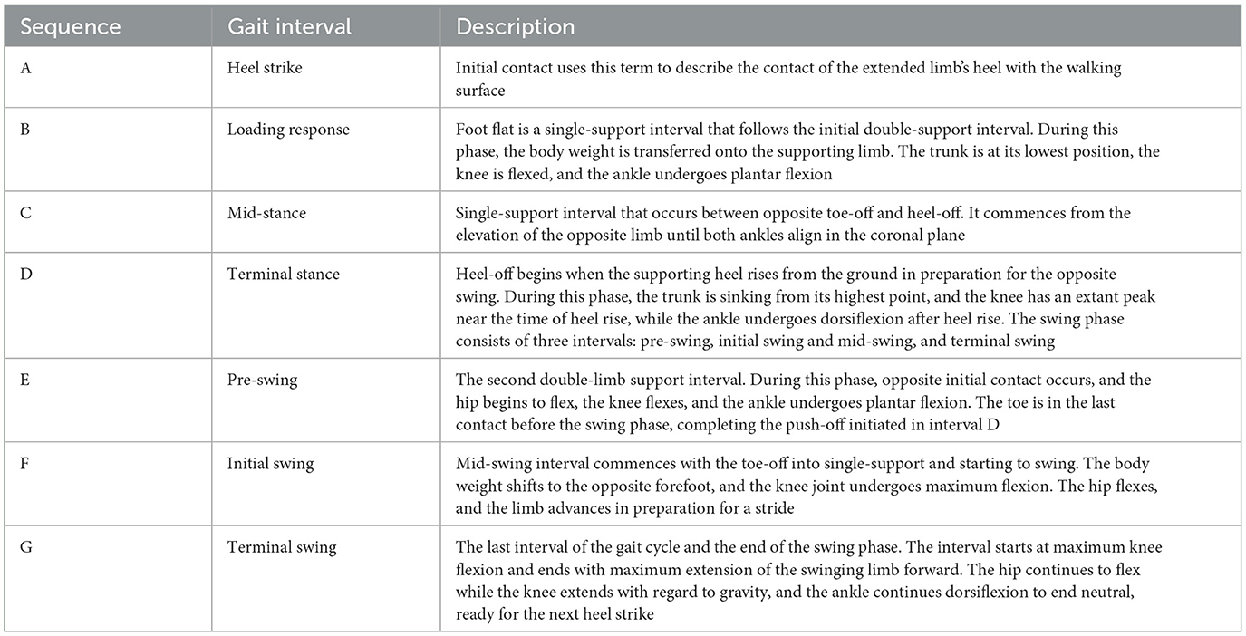
Table 1. Gait intervals.

3 Materials and methods

The categorization of gait ground reaction force (GRF) signals poses a formidable challenge, necessitating the application of sophisticated machine learning methodologies. Illustrated in Figure 2, this study delineates the framework for data acquisition and analysis. Gait data presented in Sections 3.6.1 and 3.6.2 serve as the training set for a neural network tasked with classifying these signals, and the resulting output is iteratively refined through backpropagation to pinpoint the key foot profiles crucial for classification. Detailed in subsequent sections are the experiments conducted utilizing various deep convolutional neural network (CNN) models to process and categorize spatiotemporal 3D matrices derived from raw sensor signals.

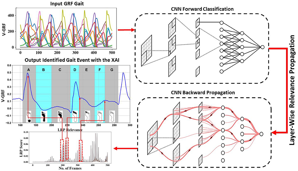
Figure 2. Overview of data acquisition and analysis of CNN. Gait data as input to CNN for classification; interpreting the CNN model by LRP, a deeper red color represents a higher contribution to the classification process. Relevance linked to the foot profile in the input single.

3.1 Convolutional neural networks

CNNs excel in classification tasks by abstracting high-level features from extensive datasets through convolutional operations. Mathematical representation in one-dimensional convolution operations is expressed as C(i), with i denoting the index of an element in the new feature map (Goodfellow et al., 2016, ch. 9):

C(i)=(ω◦ x)[i]=∑dx(i-d) ω(d)    (1)

Gait is captured as a two-dimensional signal as spatial and temporal; therefore, the convolution operation in Equation 1 can be extended to two dimensions, such that the spatiotemporal input is a large set of data points, and the kernel is a set of data smaller in size than the input. Then the convolution operation slides the kernel over the input computes elementwise multiplication and adds the values in a smaller future map. With a 2-D input x and a 2-D kernel ω with (i, j), (d, k) are iterators, the mathematical representation of convolution in two dimensions can expressed as C(i, j) with (i, j) is the index of an element in the new feature map (Goodfellow et al., 2016):

C(i,j)=(ω◦ x)[i,j]=∑d∑kx(i-d, j-k)ω(d,k)    (2)

In this study, we implement three CNN architectures for analyzing gait deterioration. The first model (Figure 3A) is a CNN designed for PD severity classification, comprising four convolutional layers, each followed by average pooling and two fully connected layers, totaling 10 stacked layers. The second CNN architecture (Figure 3B), tailored for processing GRF signals, draws inspiration from inception neural network architectures. It features two stages with parallel streams fused via concatenation layers, resulting in 18 stacked layers. The third CNN (Figure 3C) is a quadruplet network, amalgamating elements from Siamese and triplet networks. It includes convolutional layers, max-pooling, and average pooling, with separate activations, weights, and biases for each stream. This architecture aims to capture spatial and temporal gait signals simultaneously, enhancing generalization capabilities on unseen data.

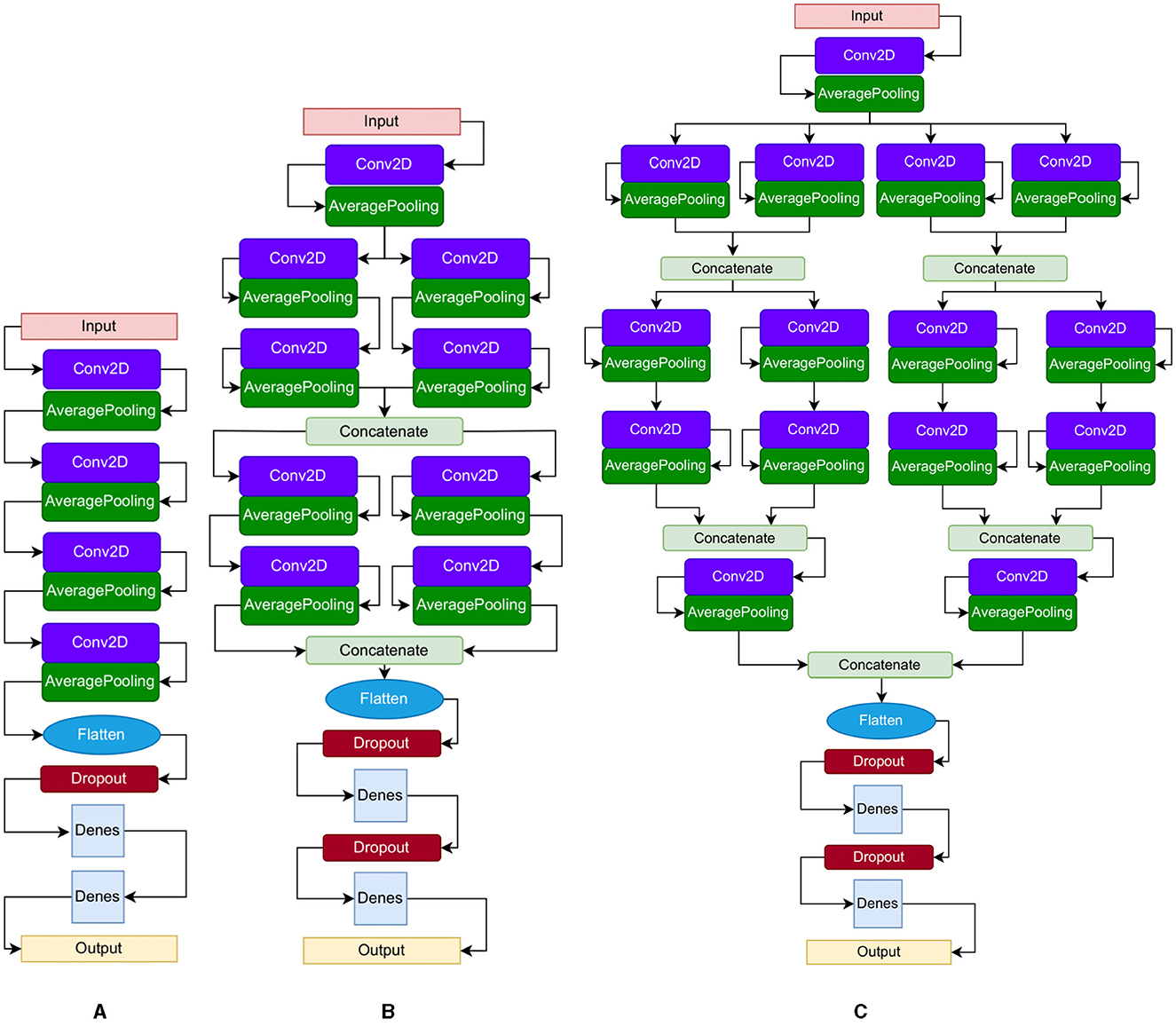
Figure 3. Proposed CNN architectures: (A) single CNN, (B) parallel CNN, (C) quadruplets CNN. The boxes: convolution layers and fully connected layers; pooling layers; concatenation layers and flattening layers; dropout layers.

3.2 Backpropagation

It is short for “backward propagation of errors”; it is an algorithm based on gradient descent. As explained by Andrew Ng (Ma et al., 2024), the method moves in reverse order from the output layer to the input layer while calculating the gradient of the error function based on the network weights, the aim is to minimize J (θ) using an optimal set of parameters in θ. It is based on performing the partial derivative to minimize the cost function. The partial derivative is expressed as ∂∂θi,jl J (θ). The output layer calculates the error of the network layers L with: d(L) = α(l)−y, such that the error of node j in layer l is denoted as dj(l) and the activation of node j of layer l is denoted as αj(l) and y is the output of the output layer, then the backpropagation can be expressed for neural networks as (Ma et al., 2024):

ð(L)=((θ(l))(T)ð(l+1))◦ α(l)◦(1−α(l))    (3)

Here, the ð* values of the output layer L are calculated by multiplying the ð* values in the next layer (in the reverse direction) with the θ matrix of layer l; hence, T denotes matrix. We then perform elementwise multiply (°) with the g′, which is the derivative of the activation function, which is evaluated with the input values given by z(l), where g′(z(l)) = α(l)°(1−α(l)).

The partial derivatives needed for backpropagation are performed by multiplying the activation values and the error values for each training example t and m is the number of training data as Ma et al. (2024):

∂∂θi,jl J (θ)=1m ⌊∑t=1mαj(t)(l)ðj(t)(l+1) ⌋.    (4) 3.3 Evaluation measure

The confusion matrix is a common accuracy measure in gait analysis (Ruuska et al., 2018). It is a table showing correct and incorrect predictions for each class, including true positive (TP), true negative (TN), false positive (FP), and false negative (F).

In this paper, we use the confusion matrix because a number of TP, TN, FP, and FN samples are values of interest to understand the confusion in gait classes for further analysis using LRP.

From this confusion matrix table, performance measures are obtained, such as accuracy, recall, precision, and F1 using the following equations.

• Accuracy: an indicator of the ratio between the correctly predicted data to the total number of samples in the dataset, defined as follows: TP+TNTP+TN+FP+FN.

• Recall: the proportion of positive classes identified correctly, defined as follows: TPTP+FN.

• Precision: the fraction of positive cases correctly identified over all the positive cases predicted, defined as TPTP+FP.

• F1-Score: the harmonic mean of Precision and Recall, defined as follows: 2*Precision*RecallPrecision+Recall.

3.4 Layerwise relevance propagation

Layerwise relevance propagation (LRP) (Bach et al., 2015; Montavon et al., 2017, 2018) is a backward propagation method used to identify the most influential parts of the input vector in the model prediction of an artificial neural network (ANN). In this thesis, we measure the contribution of individual components of the input xi (e.g., sensor signals at specific time frames) to the prediction fc(x) of a gait class c made by the CNN classifier f. The prediction is redistributed backward through the network via backpropagation until reaching the input layer. LRP generates a “heat map” over the original signal, highlighting sections with the highest contributions to the model's prediction, such as areas with the greatest variability among classes. It is important to note that a neural network comprises multiple layers of neurons, where neurons are activated as described in Montavon et al. (2018).

ak=σ(∑jajωjk +bk)    (5)

Here, ak is the neuron activation and aj is the activation of the neuron in the previous layer in a forward direction; ωjk denotes the weight received in the forward direction by neuron k from neuron j in the previous layer, and bk is the bias. The sum is computed over all the jth neurons that are connected to the kth neuron. σ is a non-linear monotonically increasing activation function. These activations, weights, and biases are learned by CNN during supervisory training. During training, the output fc(x) is evaluated in a forward pass and the parameters (ωjk+ bk) are updated by back-propagating using model error. For the latter, we base our computations on categorical cross-entropy (Zhang and Sabuncu, 2018).

The LRP approach decomposes the CNN output for a given prediction function of gait class c as fc for input xi and generates a “relevance score” R for the ith neuron received from Rj for the jth neuron in the previous layer, which is received from Rk, for the kth neuron in the lower layer, where the relevance conservation principle is satisfied as:

∑iRi←j= ∑jRj←k=∑kRk =fc(x)    (6)

The LRP starts at the CNN output layer after removing the Softmax layer. In this process, a gait class c is selected as an input to LRP, and the other classes are eliminated. The backpropagation for unspooling for the pooling layer is computed by redirecting the signal to the neuron for which the activation was computed in the forward pass. As a generalization, consider a single output neuron i in one of the model layers, which receives a relevance score Rj from a lower-layer neuron j, or the output of the model (class c). The scores are redistributed between the connected neurons throughout the network layers, based on the contribution of the input signals xi using the activation function (computed in the forward pass and updated by back-propagating during training) of neuron j as shown in Figure 2. The latter will hold a certain relevance score based on its activation function and pass its value to consecutive neurons in the reverse direction. Finally, the method outputs relevance scores for each sensor signal at a specific time frame. These scores represent a heat map, where the high relevance scores at specific time frames highlight the areas that contributed the most to the model classifications.

3.5 Perturbation analysis

Human gait, characterized by its inherent variability among individuals and even within a single individual, poses a significant challenge for developing reliable and robust models capable of accommodating such diversity in input data. Within the realm of gait analysis, layerwise relevance propagation (LRP) emerges as a promising methodology for interpreting the significance of input data points. However, the effectiveness of LRP in the context of gait analysis hinges on its resilience to noise and fluctuations in the input data stream.

To address this concern, a systematic exploration of the impact of random perturbation noise on LRP relevance scores is undertaken. This analysis serves a dual purpose: first, to inform the selection of the most appropriate LRP method, and second, to guide the design of a deep convolutional neural network (CNN) model capable of withstanding the inherent variability of gait patterns. The intricacies of this perturbation analysis methodology are elucidated in subsequent sections.

The iterative procedure proposed by Samek et al. (2017b), commonly referred to as the “greedy” approach, serves as the cornerstone for selecting the optimal LRP method and evaluating the relevance scores generated for gait classification. This iterative process involves progressively removing information from the spatiotemporal input signal, prioritizing regions with the highest relevance scores for perturbation using a “most relevant first” (MoRF) approach (Samek et al., 2017b). At each iteration, the model's performance is rigorously assessed by re-predicting test data with the accumulated perturbations. The selection of the preferred LRP method is informed by observing the most significant decline in accuracy during the initial iterations, indicating the criticality of the perturbed regions for accurate classification performance. Subsequent iterations demonstrate a slower decline in accuracy as less crucial regions are perturbed, thus providing insight into the relative importance of different input features.

Moreover, the evaluation of the significance of CNN model architecture entails a comprehensive analysis of the impact of perturbations on model performance. This process involves systematically removing the highest relevance scores obtained from the selected LRP method and evaluating the model's performance by re-predicting the test data for each perturbed model. Models exhibiting substantial performance deterioration after only a few perturbation steps are deemed most amenable to leveraging LRP. This decline in performance signifies the critical role of the removed regions in facilitating accurate classification, thereby highlighting meaningful relationships between input patterns and learned classes. Conversely, regions with minimal impact on classification performance upon removal suggest lesser relevance in discerning such relationships, thus informing subsequent model refinement efforts.

3.6 Gait data

In this paper, we investigate gait deterioration due to Parkinson's disease (PD) and under dual-task conditions (walking while performing cognitive tasks as detailed in Section 3.6.2). Specifically, we compare the effects of dual-tasking and PD on gait events. The data for this study are detailed in the following section.

3.6.1 Parkinson's disease data

In this study, we utilized the open access benchmark available on PhysioNet.org (Goldberger et al., 2003) to analyze ground reaction force (GRF) data in Parkinson's disease (PD) patients. The dataset included 93 PD patients (mean age: 66.3 years; 63% men) with varying degrees of PD progression based on Hoehn and Yahr Scale staging criteria (Frenkel-Toledo et al., 2005; Yogev et al., 2005; Hausdorff et al., 2007), as outlined in Table 2, and described in detail in Table 3. Additionally, the dataset also included GRF measurements from 73 healthy controls (mean age: 66.3 years; 55% men). During the data collection process, participants were instructed to walk for ~2 min while wearing eight sensors placed underneath each foot to measure the force [N] as a function of time. The output of the 16 sensors was recorded at a frequency of 100 frames per second. Moreover, the sum of the eight sensors of each foot was added to each subject sample along with the timestamp, resulting in a total of 19 columns. The dataset was collected by three research groups, namely the Ga group (Yogev et al., 2005), the Ju group (Hausdorff et al., 2007), and the Si group (Frenkel-Toledo et al., 2005). The sub-parts of the dataset were named after these research groups. The Ju and Si groups recorded usual healthy walking at a self-selected speed, while the Ga group included additional samples for each subject, where they performed a dual task while walking (Yogev et al., 2005). Overall, this dataset provides valuable insights into the gait patterns of PD patients and healthy individuals, which could be used to develop effective interventions for gait-related impairments in PD.

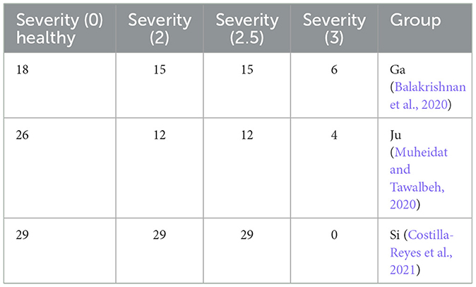
Table 2. Number of subjects with the severity rating.

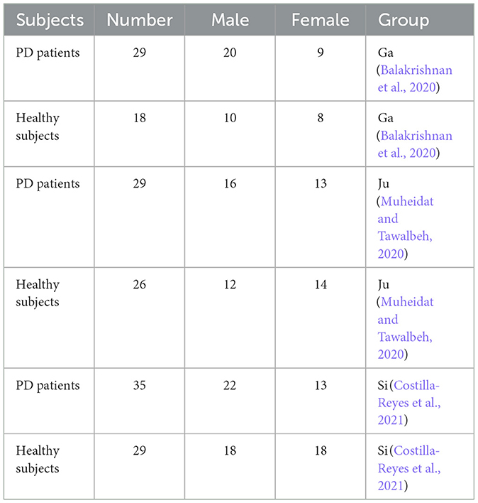
Table 3. Discerption of datasets subject.

Each sample recorded in the dataset contains 19 columns of data with varying column lengths, as for some subjects' gait was recorded for a longer time (12,119 frames) than for others (< 1,000 frames). In order to make the input data length consistent, the datasets were split into equal-size parts of 500 frames such that single long recordings are divided into several chunks of 500 frames. The timestamp columns were deleted as it doesn't report information about gait. The final sample size is 18 columns and 500 rows or frames as shown in Figure 4A. This choice is justified as the gait cycle is ~1 s, and the sample captures heel strike and toe-off for both feet over five gait cycles. The input dataset is a tensor with dimensions m × 500 × 18 where m = 2,698 for the Ga group (Yogev et al., 2005), 2,198 for the Ju group (Hausdorff et al., 2007), and 1,509 Si group (Frenkel-Toledo et al., 2005). Data standardization is performed as a pre-processing step to reduce the redundancy and dependency among the data, such that the estimated activations, weights, and biases will update similarly, rather than at different rates, during the training process. The standardization involves rescaling the distribution of values with mean at zero and rescaling the standard deviation to unity.

xn,s^=xn,s-μ(xn,s)ϑ(xn,s)    (7)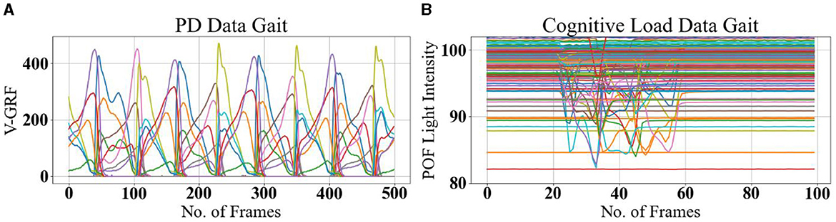

Figure 4. Example gait data. (A) PD Gait was recorded at 100 frames per second, with a sample length of 500 timeframes. The signals represent pressure sensor signals under each foot (different colors for each of the eight sensors). (B) Cognitive Load Gait, recorded at 20 frames per second, with a sample length of 100 timeframes. The signals represent POF sensors transmitted light intensity is affected by surface bending due to pressure under each foot (different colors for each of the 116 POF sensors).

Here, xn,s^ is PD data rescaled such that μ is the mean values and ϑ is the standard deviation. Then, the dataset is randomly split into training 60%, hold-out validation 20%, and testing 20% with a random state parameter with a different seed.

3.6.2 Cognitive load data

The iMagiMat footstep imaging system is an innovative floor sensor head that utilizes photonic guided-path tomography technology (Ozanyan et al., 2005; Cantoral et al., 2011; Cantoral-Ceballos et al., 2015; Ozanyan, 2015). The system can capture temporal samples from strategically placed distributed POF sensors on top of a deformable underlay of a commercial retail floor carpet in an unobtrusive manner. Each sensor is made up of low-cost POF (step-index PMMA core with fluorinated polymer cladding and polyethylene jacket, total diameter 1 mm, NA = 0.46) terminated with an LED (Multicomp OVL-3328 625 nm) at one end and a photodiode (Vishay TEFD4300) at the other. The sensors are designed to allow collaborative sensor fusion and deliver spatiotemporal sampling that is adequate for discerning gait events.

The iMagiMat system covers a 1 m × 2 m area managed by 116 POF sensors arranged in three parallel plies, sandwiched between the carpet top pile and the carpet underlay. The system includes a lengthwise ply with 22 POF sensors at 0° angle to the walking direction and two independent plies, each consisting of 47 POF sensors, arranged diagonally at 60 and −60°, respectively (see Cantoral-Ceballos et al., 2015, for the iMAGiMAT system). The system is managed by electronics contained in a closed hard-shell periphery at carpet surface level and is organized into eight-channel modules, including LED Driver boards and input trans-impedance amplifier boards to receive the data and send it to a CPLD (complex programmable logic device) to reformat the data for processing by a Raspberry pi single-board computer for export via Ethernet/Wi-Fi. The operational principle of the system is based on recording the deformation caused by the variations of ground reaction force (GRF). As bending affects the POF sensors, transmitted light intensity is affected by surface bending. This captures the specifics of foot contact and generates robust data without constraints of speed or positioning anywhere on the active surface.

For this experiment, 21 physically active subjects aged 20–40 years, 17 men and four women, without gait pathology or cognitive impairment, participated. The study was carried out under the University of Manchester Research Ethics Committee (MUREC) with ethical approval number 2018-4881-6782. All participants were informed about the data recording protocol according to the ethics board's general guidelines, and written consent was obtained from each subject prior to the experiments. Each participant was asked to walk normally or while performing cognitively demanding tasks along the 2 m length direction of the iMagiMat sensor head. The captured gait data was unaffected by start and stop, as it was padded on both ends with several unrecorded gait cycles before the first footfall on the sensor. With a capture rate of 20 timeframes/s (each timeframe comprising the readings of all 116 sensors), experiments yielded 5 s long adjacent time sequences, each containing 100 frames. The recorded gait spatiotemporal signals were able to capture ~4–5 uninterrupted footsteps at each pass.

A dual-task gait test detects mild cognitive impairment (Wang et al., 2023); therefore, five manners of walking were defined as normal gait plus four different dual tasks, and experiments were recorded for each subject, with 10 gait trials for each manner of walking in a single assessment session. Thus, the total number of samples is 10 × 5 = 50 per-subject. The five manners of walking are defined in Table 4. A set of measured data as xn,s=[xn,1&…&xn,116]∈ℝn×116is harvested from the iMagiMat system, where n is the number of the data block (100 frames) and s enumerates the POF sensors, as shown in Figure 4B. A total number of 1, 050 samples are recorded for 21 subjects and placed in a 3D matrix of dimensions 1, 050 × 100 × 116. The recorded amplitude of data varies due to the weight of each subject; therefore, data standardization is implemented as a pre-processing step, to ensure that the data are internally consistent, such that the estimated activations, weights, and biases update similarly, rather than at different rates, during the training process and testing stage. The standardization involves rescaling the distribution of values with a zero mean unity standard deviation, using Equation 7, where xn,s^ is gait data rescaled so that μ is the mean and ϑ is the standard deviation. Then, the dataset is randomly split into training 60%, hold-out validation 20%, and testing 20% with a random state parameter with a different seed.

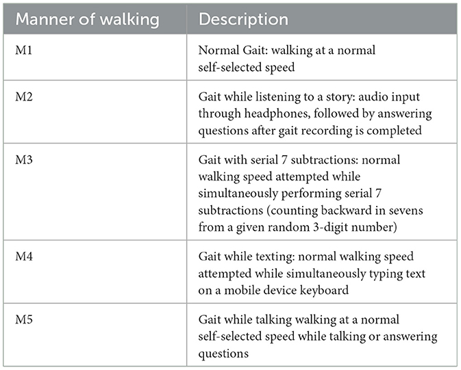
Table 4. Cognitive load experiment data.

4 Experiment and results

All algorithms for LRP computation are implemented in Python 3.7.3 programming language using Keras 2.2.4, TensorFlow 1.14.0, and iNNvestigate GitHub repository (Alber et al., 2018). The codes are executed on a desktop with Intel Core i7 6700 CPU @3.4 GHz. The deep CNN model is applied to the datasets to test the validity of the algorithms for identifying gait signatures. The implementation and the perturbation analysis are detailed in the following section. We compare the CNN predictions to manually labeled ground truth in several experiments, including PD severity staging, individuals' identity, and the effects of cognitive load on normal gait. The models' classification performance is evaluated using confusion matrices. The performance of the LRP methods is examined in detail in the discussion subsection.

4.1 Classification experiments