In this article, we combined the efficient learning algorithm of LightGBM with the automated hyperparameter optimization capability of Optuna to form a diabetes prediction framework. This section mainly introduces the mathematical description, architecture, and methods of this model.

Mathematical description

Diabetes prediction can be viewed as a binary classification problem. Given a dataset \(D=_,_\right)\right\}}_^\), where \(_\) is the feature vector of the \(^}\) sample, and \(_\in \left\\right\}\) is the corresponding label. The goal is to train a model \(f\left(x\right)\) to predict the label of unseen samples.

LightGBM Model

LightGBM is a tree-based learning algorithm that optimizes many aspects of traditional Gradient Boosting Decision Trees (GBDT) [20]. LightGBM, when handling large-scale datasets and complex models, can train models faster and more efficiently than traditional GBDT algorithms while maintaining high prediction accuracy. The prediction value \(f\left(x\right)\) of a LightGBM model can be represented as the weighted sum of multiple decision trees:

$$f\left(x\right)=_^__\left(x\right)$$

(1)

where \(K\) is the number of decision trees, \(_\left(x\right)\) is the prediction result of the \(^}\) decision tree, and \(_\) is the weight of the \(^}\) tree.

The key to LightGBM lies in its optimized approach to data handling and decision tree construction. It employs a histogram-based algorithm to accelerate the training process and reduce memory consumption, and uses a leaf-wise growth strategy to enhance model accuracy.

Optuna hyperparameter optimization

Optuna is an automated hyperparameter optimization framework, whose core is to search for the optimal parameter combination by defining an objective function to minimize or maximize its value [21]. In the LightGBM model, Optuna can be used to find the optimal hyperparameters, such as num_leaves, max_depth, learning_rate, and others. In the Optuna-LightGBM-based diabetes prediction model, the hyperparameter combination with the highest cross-validation score is selected.

$$_=_\left(\right)}$$

(2)

Where \(_\) is the parameter set that maximizes the cross-validation score \(C_}\). \(C_\left(\right)}\) is the cross-validation accuracy score given a parameter set. The \(p\) represents the parameter set of the model, including but not limited to num_leaves, max_depth, and learning_rate.

During the optimization process of Optuna, it automatically tests multiple different parameter combinations. Each set of parameters is evaluated based on its cross-validation score, and the evaluation results determine which set of parameters can provide the best model performance. This process is based on the results of previous experiments to guide the direction of subsequent searches so that the optimal parameter configuration is to be found in the shortest possible time.

Model architecture

In this article, the diabetes prediction dataset from ‘kaggle’ was used, which contains 9 attributes and 100,000 records. The detailed description of the dataset is provided in Table 1.

Table 1 Data description of the diabetes prediction dataset.

The nine attributes are gender, age, hypertension status, history of heart disease, smoking history, BMI, glycated hemoglobin level, blood sugar level, and the output result. The output result represents the diabetes status of each individual data point, while the other variables are independent feature variables. Among the 100,000 samples, there are 8,500 patients with diabetes and 91,500 patients without diabetes. The proportion of patients with diabetes is only 8.5%, significantly lower than the 91.5% of non-diabetic patients, making the dataset highly imbalanced.

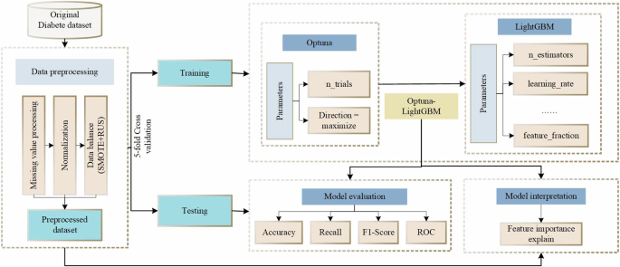
For effective improvement of the prediction performance of the unbalanced diabetes prediction dataset, Optuna is used to optimize the LightGBM performance parameters, The detailed process of Optuna-LightGBM model is depicted in Fig. 1.

Fig. 1

Overall design of the proposed model.

In the Optuna-LightGBM-based diabetes prediction model, data preprocessing, which includes data cleaning, feature engineering (feature selection, feature transformation, etc.), and missing-value processing, is performed first to ensure data quality and improve model performance. Then, data resampling technique (SMOTE + RUS) is used to deal with the data imbalance. Next, a hyperparameter search is performed to automate the search for the optimal hyperparameters of the LightGBM model with Optuna, a step that is achieved by defining the search space, the optimization objective and the cross-validation strategy. Finally, model training, which uses Optuna-optimized hyperparameter settings to train the model with the LightGBM algorithm, and evaluates the model performance with cross-validation methods to select the optimal Optuna-LightGBM model for prediction.

The proposed method of Optuna-LightGBM

When utilizing Optuna for hyperparameter optimization, the first step is to define the search range for each hyperparameter, such as setting the range of values for parameters like learning rate and maximum tree depth. Next, an objective function is designed to measure the performance of the model given the hyperparameters by evaluating the performance metric, accuracy, on the validation set. Through this target function, Optuna can explore the hyperparameter space, iteratively trying different parameter combinations, and adjusting its search strategy based on performance feedback to ultimately determine the best hyperparameter configuration that optimizes model performance. LightGBM parameter settings are shown in Table 2.

Table 2 Parameters setting of the LightGBM.

When training the LightGBM model, the model is initialized according to the optimal parameter settings provided by Optuna. To solve the problem of data imbalance, the SMOTE + RUS balancing technique was adopted for resampling the training data to improve the data distribution during model training. Subsequently, the LightGBM model was trained on the adjusted data, and a series of decision trees were constructed step by step using the gradient boosting technique to minimize the prediction error. Finally, the performance of the model is evaluated through cross-validation, which uses metrics such as accuracy, recall and F1 score to assess the prediction accuracy of the model.

The proposed model’s workflow diagram is shown in Fig. 2. The sharing of parameters between different modules in the diagram enables the model to learn global features better, thereby improving model prediction efficiency and generalization ability. With the aforementioned methods, the diabetes prediction model based on Optuna-LightGBM achieves high accuracy in predicting diabetes risk, which provides a strong support for clinical decision-making.

Fig. 2

Flowchart of the proposed method for prediction.

The algorithm flow for balancing the dataset using SMOTE and random under-sampling, followed by training and optimizing the LightGBM model with Optuna, is given as follows.

Algorithm 1. Pseudocode of the Improved LightGBM.

Data preprocessing

In machine learning, the quality of input data has a significant impact on the output results, and it is necessary to preprocess the existing dataset before making predictions. Therefore, we need to clean the data to avoid inaccurate prediction results and reduce the misclassification rate of the predictive model. Furthermore, it is also essential to analyze the distribution of the dataset and process the unbalanced dataset through data balancing algorithms that increase the model’s perception of the few categories of data and improve its robustness.

Data cleansing

Data cleansing, a crucial step in the data preprocessing phase, is instrumental in achieving data integrity. It involves addressing missing values, eliminating duplicates, and correcting inconsistencies or errors. With it we can significantly reduce the likelihood of biased or inaccurate results in our analyses.

An initial check for missing values in the dataset was performed. By carefully evaluating the presence of “No info” values and making decisions regarding predictors with a high proportion of missing values, we aim to maintain the integrity and quality of the dataset. This approach ensures more reliable analysis and accurate interpretation. The distribution of the cleaned dataset is shown in Fig. 3.

Fig. 3

Distribution of cleaned datasets.

Figure 3 presents the kernel density distribution plots for each attribute of the diseased and non-diseased categories along the main diagonal. The upper triangle shows scatter plots of each attribute’s distribution for the two categories, while the lower triangle displays marginal kernel density plots (contour plots) for the attributes of the two categories. It can be observed that in the cleaned dataset, the kernel density distribution trends for diabetic and non-diabetic samples are quite consistent for attributes such as age, hypertension, heart disease, and BMI. However, the distribution differences are more pronounced for HbA1c levels and glucose levels. In the scatter plots and marginal kernel density plots, there is a certain degree of overlap between the samples of the two categories, but overall, the boundaries of the distribution areas for the two categories are relatively clear. This indicates good separability, which is beneficial for training and predicting with the diabetes prediction model.

Data splitting

The performance of machine learning models largely depends on data quality and data strategies [22]. Therefore, it is important to evaluate the impact of data splitting on the performance of machine learning models. The data splitting methods used in this article include K-fold cross-validation and random splitting using the train-test split method.

K-fold cross-validation is a statistical technique used to evaluate the performance of machine learning models. This method divides the dataset into K equally sized subsets. Among these K subsets, each subset is used in turn as the test set, while the remaining K-1 subsets are combined to form the training set for model training. This process is repeated K times, with each iteration selecting a different subset as the test set and the rest as the training set. Ultimately, performance evaluation results for K models are obtained. This process iterates based on the number of folds. The model’s generalization performance is estimated by averaging the obtained scores [23], as shown in Fig. 4a.

Fig. 4: Data splitting methods.

a Performing k-fold cross-validation. b The dataset is divided into two parts randomly with different ratios: 80: 20, 70:30, and 60:40 train/test split.

The train-test split method divides the dataset into random training and testing subsets. This approach depends on the size of the dataset [24], as shown in Fig. 4b.

Correlation analysis

A correlation matrix is used to analyze the relationships among various attributes in the cleaned dataset by statistically calculating the connections or relationships between two or more variables in the dataset. This relationship is measured numerically, with higher values indicating a closer relationship between the inputs and desired outputs. The correlation matrix of the diabetes prediction dataset is shown in Fig. 5.

Fig. 5

Correlation matrix heat map.

From the correlation matrix heatmap in Fig. 5, it can be seen that HbA1c levels, glucose levels, and age have a closer relationship with the output results in the cleaned dataset. In the diabetes prediction dataset, the attributes do not show a clear tendency to covary with each other, and there is no high correlation of strong covariance. Additionally, a low correlation of a feature only means that the feature is not useful in the presence of other features, but it does not imply that the feature is unimportant for predicting diabetes. In conclusion, the predictors in the diabetes prediction dataset did not show a significant correlation. Therefore, there is no need to worry about high correlations affecting model performance or introducing bias.

Data augmentation

In the diabetes prediction dataset, the data for diabetic patients accounts for only 8.5%, which is <10%, indicating a highly imbalanced state. To balance the class imbalance in the existing dataset, a combination of SMOTE oversampling and RUS undersampling methods is used.

The SMOTE algorithm is an improved solution based on the random oversampling algorithm proposed by Chawla [25], which is a method for oversampling synthetic minority class samples. Since the random oversampling technique simply duplicates samples to increase the minority class samples, it may lead to overfitting issues, where the model learns overly specific information and lacks generalization. The basic idea of the SMOTE algorithm is to analyze the minority class samples and synthetically generate new samples to be added to the dataset.

In an imbalanced dataset, where the set of minority class samples is denoted as \(_}\), the core idea of SMOTE is to interpolate between minority class samples to augment those with fewer data points, thereby balancing the number of samples for different labels. For each sample \(_\) in \(_}\), the k-nearest neighbors method is used to find a sample \(_\).Then, for each pair of \(_\) and \(_\), the difference vector d = xi–xi is calculated, and a new sample \(_}\) is generated. The expression for \(_}\) is as follows:

$$_}=_+\left(0,1\right)\times \left(_-_\right)$$

(3)

where \(\left(\mathrm\right)\) represents a random number within the range (0,1).

The SMOTE algorithm synthesizes new minority class samples to increase the quantity of minority class samples, retaining the information of the original data. However, it does not process the majority class samples, which may result in the loss of some majority class information. The RUS Random undersampling refers to the process of removing some samples from the majority class to reduce redundancy and achieve data balance.

If the set representing the majority class samples is denoted as \(_}\), then the process involves calculating the number of majority class samples to retain, denoted as \(M\), typically approaching or equaling the quantity of minority class samples. Subsequently, M samples are randomly selected from Dmajority.

The combined use of SMOTE and RUS involves first applying SMOTE to increase the number of minority class samples and then performing RUS to decrease the number of majority class samples. Assuming \(N\) is the desired number of new minority class samples, the objective of this combined method is to create a new dataset where the number of samples in the minority and majority classes is more balanced.

The process of combining SMOTE and RUS can be outlined in the following steps:

1.

Apply SMOTE to generate new minority class samples \(_}^ }\) until the quantity reaches \(N\).

2.

Perform random undersampling from the majority class \(_}\) to obtain \(_}^ }\).

The final synthesized dataset \(_}\) is obtained by merging \(_}^ }\) and \(_}^ }\)’:

This combined approach allows fine-tuning of the class balance of the new dataset by adjusting \(N\) and \(M\).

Evaluation index

Given that the accuracy of predicting diabetic patients has a greater impact than that of non-diabetic patients, this article uses the confusion matrix and the receiver operating characteristic (ROC) curve [26] as experimental evaluation metrics. Note that in diabetes prediction, more attention is paid to the accuracy of predicting diabetic patients, aiming to minimize false negatives (predicting diseased as healthy). The evaluation metrics from the confusion matrix are listed in Table 3.

Table 3 Model evaluation based on binary confusion matrix.

The data in the confusion matrix are used to estimate a set of statistically relevant performance indicators defined as follows.

$$\text=\frac+}+++}$$

(5)

In the ROC curve, the true positive rate (TPR) is plotted on the y-axis and the false positive rate (FPR) is plotted on the x-axis. The TPR is mathematically the same as the recall rate, whereas the FPR indicates how many false positives occurred out of all the available negative samples during the testing period. The formulas for calculating the TPR and FPR are as follows: