Activity meter and source assessment

SPECT/CT calibration requires samples with well-known activity. Accordingly, having access to an activity meter that is traceable to a national or international standard is crucial for accurate calibration. In this study, a Veenstra VDC-505 m (Veenstra, Joure, The Netherlands) was used to assess the samples used. This meter undergoes regular quality control, including comparisons to standards. Since the scope of this study was count-rate management in calibration rather than system calibration itself, it was not considered necessary to use a 131I reference source for calibration close in time to the study. However, based on comparisons to traceable standards at other occasions, the accuracy in 131I measurements is estimated to about 2%. Stability controls performed daily over several years using a 7 MBq 137Cs source indicate a precision below 3%.

In this study, all sources were only measured once with the activity meter. Since accurate relative activity was considered most important for the aims of this study, it was selected to (i) base phantom activity on physical decay, and (ii) consistently use the same sources and phantoms for the two SPECT/CT systems.

SPECT/CT systems

The data presented in this paper were collected with two GE Discovery 670 Pro SPECT/CT systems (GE Healthcare, Haifa, Israel), which exhibit the characteristics of a paralysable data acquisition system. According to personal communication with a GE representativeFootnote 1, front-end-electronics block pulses that are too close in time in order to prevent pile-up effects, efficiently manifesting as a dead time τ per detector pulse of 1.6 μs in the standard setting. However, pileup from two pulses close enough in time to be indistinguishable must still be expected despite this functionality.

The SPECT/CT measurements were performed using the High Energy General Purpose (HEGP) collimators, and the reconstructions were executed on a Xeleris workstation using the Volumetrix MI Evolution software. However, it is expected that the procedures presented in this paper are applicable to any SPECT/CT system and any reconstruction software.

Energy settings

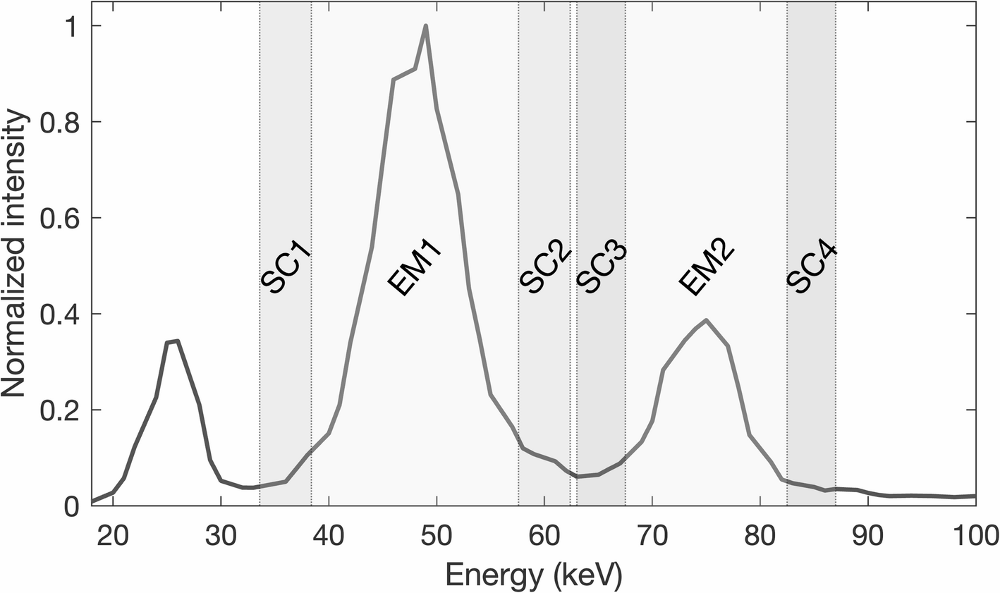
Because dead-time and pulse-pileup losses depend primarily on the total number of pulses in the detector, energy protocols were defined to cover the total available energy range, in addition to an 131I-specific triple-energy window (TEW) protocol. The energy protocols used are presented in Table 1.

Table 1 Energy protocols used in this work

The Discovery 670 Pro system’s “high energy” option was applied, widening the available energy range from the standard [0,512] keV to [0,681] keV, thus enabling the use of the “Open_HE” protocol.

Planar measurementsAssessment of system dead time

The dead time per detector pulse was determined for each detector head of the two SPECT/CT systems using the two-source method [9], with the purpose to independently validate the manufacturer-given value. Two syringes were prepared with 131I activities of 49.2 and 49.9 MBq. These were placed in the point-source position assigned for control of intrinsic uniformity, more than 3 m from the surface of the detector. Measurements were performed without collimation, using the so-called intrinsic collimators, i.e. plastic covers that protect the detectors. The two 131I sources were measured separately and in combination, resulting in total spectrum count rates R1, R2 and R12, respectively, collected using the Open_HE energy protocol (see Table 1). The system dead time was given by Eq. (1), assuming a paralysable system:

$$\:\tau \: = \frac}}} + } \right)}^2}}} \cdot \:ln\left( + }}}}}} \right)$$

(1)

The response of a paralysable data acquisition system is defined by Eq. (2), describing the relation between the observed spectrum count rate, Rout, and the true pulse rate, Rin, depending on the dead time per pulse, τ.

$$\:} = } \cdot \:} \cdot \:\tau \:}}$$

(2)

To get the true number of detector events, a dead-time correction factor CDT = Rin/Rout must thus be applied to the measured number of counts. Because Eq. (2) does not allow an analytical solution for Rin, a four-degree polynomial approximation PDT(Rout) was adopted in this work to express CDT as a function of Rout. This is further described in the results section.

Assessment of count losses from dead time and pulse pileup

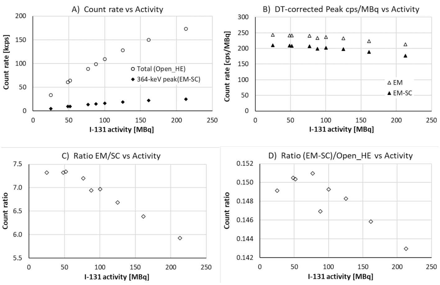
A set of intrinsic planar measurements, thus not using collimation, was performed for one detector head with the purpose of visualising how count losses from dead time and pulse pileup manifest at various count rates. For these measurements, four syringes were prepared with 131I activities of 25.0, 48.6, 51.9 and 88.2 MBq, totalling 213.7 MBq. These were placed more than 3 m from the surface of the detector one at the time and in various combinations. When used in combination, the syringes were placed > 2 cm apart to limit scattering.

Data were collected using both energy protocols in Table 1. Information on changes in the energy spectrum, expected due to pulse pileup, was extracted by analysing the ratio of counts in the emission and scattering windows of the 364.5 keV peak (EM/SC) and the ratio of scatter-corrected counts in the 364.5 keV window to the total spectrum counts ((EM-SC)/Open_HE).

In this study, the pileup losses in the 364.5 keV energy window were investigated, using the scatter-corrected counts (EMSC). The data were related to the total spectrum count rate, recorded using the Open_HE energy protocol, and corrected for dead-time losses using the polynomial PDT(Rout) obtained from the dead-time assessment. Any remaining differences between measured and expected count rates were attributed to losses due to pulse pileup. In this procedure, known source contents were used while assigning correction factors CPU to maintain constant (EM-SC) count rate per activity unit. For all data, background counts were subtracted, averaged from recordings without any source present before and after the source measurements. The time for all acquisitions was 60 s.

For presentation purposes, a third-degree polynomial fit PPU(Rout) was made to the obtained CPU data, which is further described in the results section. The uncertainties of the underlying data points are dominated by uncertainties in measured 131I activities, estimated to 2–3%. Uncertainties emanating from counting statistics were a magnitude smaller.

Assessment of extrinsic planar sensitivity

A basic 131I calibration measurement involves measuring the planar sensitivity using a point-like source or a Petri-dish source, albeit this type of calibration is claimed to be of doubtful use for SPECT/CT quantification [1, 3, 5]. In this study, extrinsic point-source planar-sensitivity measurements were performed for the purpose of obtaining a rough comparison with data obtained in SPECT/CT calibration. Three point sources (syringes) with a content of 12.3, 21.7 and 31.7 MBq 131I were placed consecutively between the two detectors, with the HEGP collimators mounted, and planar images were collected for 60 s.

Analyses of the sensitivity were performed using the I131TEW scatter corrected data (referred to as EM-SC), and total spectrum count rates were assessed using the Open_HE data (Table 1). The energy spectrum count rate was kept low enough to maintain a dead time of < 1.5%, although dead time corrections were applied. Background measurements were also performed and subtracted. Uncertainty estimates for the system sensitivities were calculated based on measurements of the three 131I sources and the two detectors of each system. In addition, the size of the image region subject for analysis was varied, allowing for analyses of its influence on measured sensitivity for the two systems.

Tomographic phantom measurementsObjects under study

SPECT/CT measurements were performed on two phantoms at 11 occasions per phantom over a time period of two months, June-August and October-December 2022, respectively;

(A)

A homogeneous water-filled Jaszczak phantom with an initial 131I activity of 2160 MBq and a final activity of 16 MBq;

(B)

A cold water-filled Jaszczak phantom with a hot 6 cm diameter spherical insert, which was filled with an initial 131I activity of 2090 MBq and a final activity of 9 MBq.

To enable use of activity concentrations, the water volumes were assessed by measuring the weight before and after filling of phantoms as well as insert. Before adding 131I, potassium iodide was introduced to block the activity from attaching to the walls of the phantom and insert, respectively.

The long time of assessment enabled analyses over a wide range of system count rates. In this study, precision of relative activities was considered more important than the accuracy of absolute activities, governing the choice of repeated measurements over time, rather than filling the phantoms with gradually more activity. Whereas the accuracy of the absolute activities of the phantoms was limited by the accuracy of the activity meter, the uncertainties in relative activities in each set of phantom measurements were thus governed by physical decay only, leaving only a minor error from precision in the 131I half-life. Here a value of 8.0252 days was used [10].

Data collection and reconstruction

Both phantoms were measured using both SPECT/CT systems, producing a total of four data sets. All data were collected using clinical SPECT/CT protocols with the HEGP collimators and the I131TEW energy setting (see Table 1). The matrix size was 128 × 128 pixels, the auto-contour option was applied, and no zoom was used. Each SPECT data collection of phantom (A) comprised in total of 90 projections, collected for 8 s per projection, and was followed by CT data acquisition. Phantom (B) was assessed using 72 projections, collected for 25 s per projection. The change in the data collection scheme between phantoms was unintentional and occurred due to a change in clinical practice between the measurement series. The 2.5 times longer data collection for phantom (B) was reflected in a proportionally larger number of collected counts.

For phantom (A), data collection and analysis were repeated three times at each measurement occasion to deduce information on random uncertainties. The phantom was removed and replaced between each data collection. Keeping the data collection times constant over the measurement series implied a lower number of collected counts at lower phantom activities, thus larger random uncertainties were anticipated at lower activities. For phantom (B), no repetitions were made, motivated by previously recorded data showing that random uncertainty was subordinate to systematic differences emanating from variations in count rate.

In connection to every phantom measurement, the total spectrum count rate over a set of projection angles was also assessed using the Open_HE energy protocol (see Table 1). These data were collected to establish and utilise a relation between the average total spectrum count rate and counting losses in the 364.5 keV energy window due to dead time and pulse pileup. This procedure is further described below. Finally, background measurements were also collected, using an inactive Jaszczak phantom.

The reconstructions were executed using the clinic’s dedicated dosimetry reconstruction protocol, denoted as IRACSCRR in Xeleris. It is an OSEM iterative reconstruction (IR) scheme, applied with 10 subsets and 10 iterations, which adopts CT-based attenuation correction (AC), scattering correction (SC) and resolution recovery (RR). For comparison, some reconstructions were also executed when turning the resolution recovery option off, resulting in a reconstruction alternative denoted as IRACSC.

The series of measurements on phantom (A) were used to establish tomographic dead-time and pulse-pileup corrections as well as to perform a tomographic sensitivity calibration. The series of measurements on phantom (B) were used to control the applicability of the loss-correction scheme from (A) and to identify a robust procedure for regular calibration control.

Correcting for dead time and pulse pileup

In tomographic measurement and reconstruction, corrections for dead time and pulse pileup are more complicated than in planar measurements, because the projections are collected using two detector heads at various count rates. Consequently, accurate accounting for losses would require individual corrections for each projection. However, a typical contemporary SPECT/CT system does not provide the possibility to correct each projection individually, wherefore the user is left with the possibility to make a general correction to the complete data set. Alternatively, the user may develop more advanced self-build analysis tools, which falls beyond the scope of this work.

In this work, the following procedure was adopted for correcting tomographic 131I measurements for count losses;

i.

Executing a series of SPECT/CT measurement of a homogeneous Jaszczak phantom with a range of known source contents of 131I, while collecting data using the Open_HE and the I131TEW energy protocols (see Table 1);

ii.

Analysing the ratio between the total number of background-subtracted, scatter-corrected 364.5 keV energy window counts (EM-SC) in all projections and the 131I activity at the time of each SPECT acquisition;

iii.

Defining a dead-time and pulse-pileup correction factor CDTPU(Rout) for each data point, which returned a constant number of peak counts per activity unit, equal to the projected counts per MBq at the 0 MBq limit;

iv.

Fitting a four-degree polynomial PT(Rout) to the obtained CDTPU(Rout) data, using the boundary condition PT(0) = 1. In this step, a subjectively selected limit in count rate was introduced to at Rout = 160 kcps, where about 50% losses were encountered;

v.

Using the PT(Rout) polynomial to correct the number of counts in reconstructed image stacks for dead-time and pulse-pileup losses based on the total spectrum count rate.

One may note that the correction scheme will only be valid up to the limit of Rout selected in the polynomial fit, which was 160 kcps in this work, and data points above this limit should be considered unreliable.

In this study, ratios of counts in the adopted energy windows were also used to provide information on changes in the energy spectrum due to pulse pileup. The adopted ratios were the same as in the planar measurements; (EM/SC), i.e. the ratio of counts in the emission and scatter windows of the 364.5 keV peak, and; ((EM-SC)/Open_HE), i.e. the ratio of scatter-corrected counts in the 364.5 keV window to the total spectrum counts.

Determining the SPECT/CT sensitivity

The reconstructed image stack may be used for calculating the SPECT/CT sensitivity using three methods;

(a)

Using all voxel counts in the complete image stack, or full field of view (FOV), here called Full-FOV data, and calculating the sensitivity as the total number of counts per second per source unit [cps/MBq];

(b)

Using the voxel-count concentration over a central region of the source and calculating the sensitivity by dividing with time and the source concentration [(cps/ml)/(MBq/ml)];

(c)

Delineating the source in the image stack and calculating the sensitivity as the number of counts in the delineated object divided by time and its source content [cps/MBq].

Data from the homogeneous phantom (A) were used for determining the SPECT/CT system sensitivity. Calculation methods (a) and (b) were applied, which are expected to return similar values. Method (c) is expected to return a lower value due to imperfect spatial resolution and resulting partial-volume effects, and it was thus not used on data from phantom (A). However, this method is still relevant for regular calibration controls (see below).

The series of measurements allowed for assessment of how the level of phantom 131I activity influences the results. Whereas background counts may be considered negligible at moderate or high count rates, the scope of this study also included low count rates. Accordingly, all SPECT/CT data presented in this work included subtraction of background counts, which were obtained in measurements of an inactive, water-filled Jaszcak phantom. The background images were collected, reconstructed and analysed using the same settings as the active phantom data.

Verifying the calibration factor

Once the calibration factor (CF) has been determined, its consistence over time must be controlled regularly. In this article, such controls are suggested to be performed using phantom geometry (B), i.e. a Jaszczak phantom with a centrally placed spherical insert, which contains the activity to be assessed. The main advantages of using such a geometry are; (i) only the spherical insert is activated, leaving the Jaszczak phantom available for other quality control after the measurements, (ii) a spherical insert offers fast and practical delineation in reconstructed image stacks, and; (iii) as compared to other geometries with an insert or vial source, a central sphere provides data collected at fairly constant projection count rates, limiting errors that emanate from the lack of possibility to perform dead-time and pulse-pileup corrections on individual projections.

For the data collected using phantom geometry (B), all three sensitivity-calculation methods (a)(c) were used, allowing for assessment of how the level of 131I activity in the insert influences the results for each calculation method. One should bear in mind that method (c) will result in a lower sensitivity value because of partial-volume effects. Still, this method may be applicable for controlling the consistency of calibration over time.