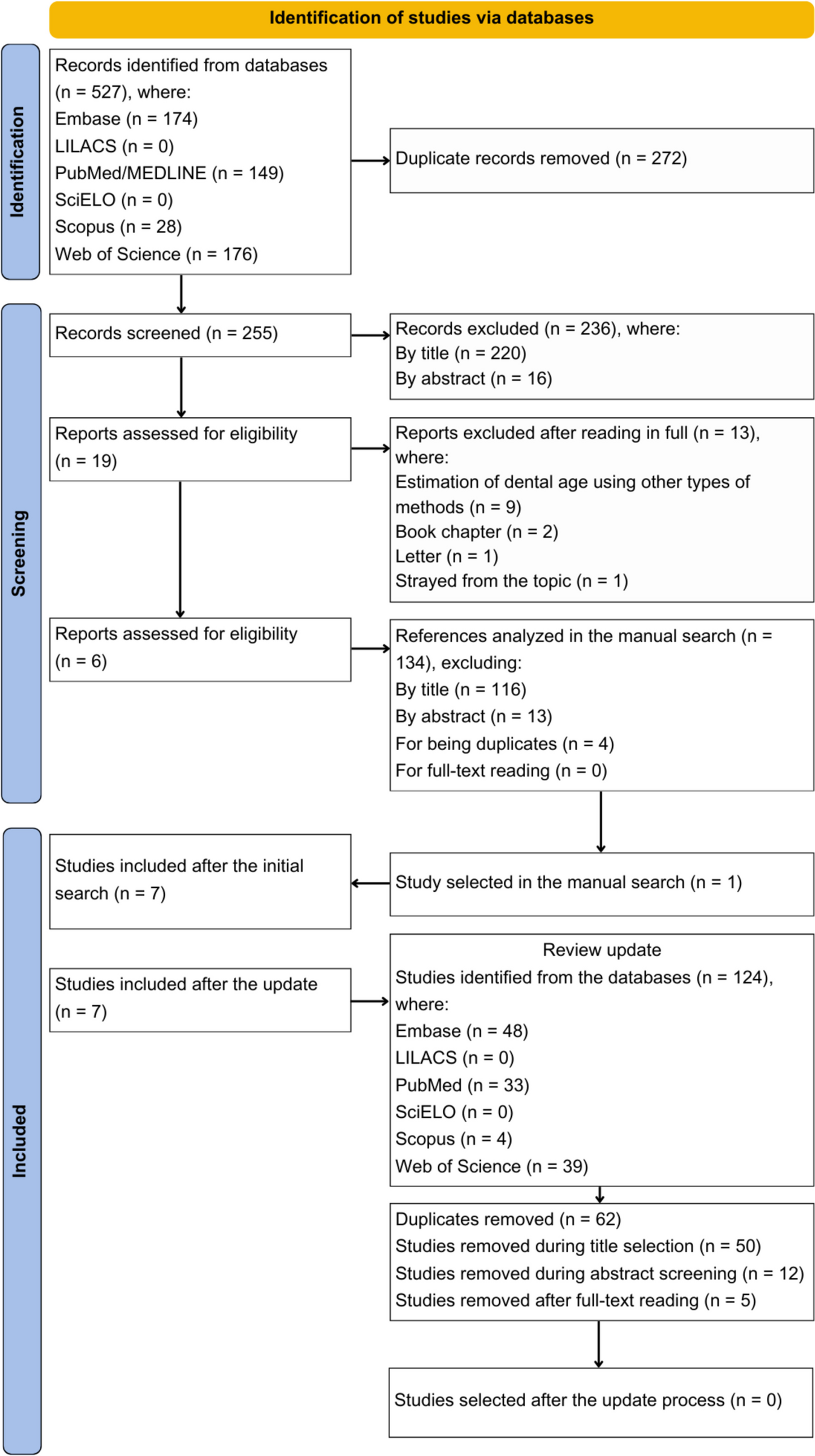
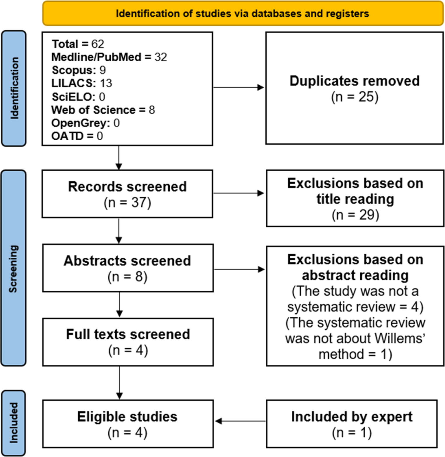
In Sweden, medical-legal autopsies are conducted at one of six forensic medicine units of the National Board of Forensic Medicine (NBFM). We searched the NBFM autopsy database from 2001 to 2021 for non-homicide decedents aged 18 years or older who had undergone an autopsy (n = 105 952), where the registered underlying cause of death was liver laceration (n = 102) (Fig. 1).

A flow chart showing how cases were selected and excluded/included

We reviewed each autopsy report and excluded cases where the underlying cause of death as recorded in the autopsy report was not liver laceration only, e.g. where the cause of death was a combination of injuries (n = 79), as well as cases that had received hospital care (n = 4), leaving 19 cases (Fig. 1). For these cases, we extracted injuries, height, weight, sex, and measured blood volumes in the body cavities, as well as signs of hypovolemic shock, that is, pale lividity, as well as kidney pallor, lung pallor and/or subendocardial haemorrhage. Further, we also extracted information about known disease and autopsy findings of incidental disease.

As in the inciting study we calculated total blood volume using Nadler-Hidalgo-Bloch and Lemmens-Bernstein-Brodsky and Friesen Eqs. [11,12,13], the latter using Friesen’s altered versions of Janmahasatian’s lean-scale-factor [14] (Table 1). As in the inciting study, we also use the experience-based methods of assuming a total blood volume of 7–8% of body weight [6] (Table 1).

As noted in the inciting study [6] there are many issues with finding accurate measures of intra-abdominal blood volume (IABV): (I) the presence of both internal and external haemorrhage in many cases, making it difficult, if not impossible, to correctly estimate total blood losses, (II) the impact of resuscitation attempts including causing additional injuries as well the addition of blood or other fluids during resuscitation, which can artificially inflate haemorrhage volume, (III) coexisting pathology limiting haemorrhage volume (as compared to some hypothetical healthy case), (IV) some blood volume being unmeasurable as it is within surrounding tissue, and (V) error in measuring the measurable proportion of internal haemorrhage.

Issue I is alleviated through case selection while issue II can be solved via conducting separate analyses. Regarding the issue of coexisting pathology raised in III we are of the opinion that it is not an error at all but merely a representation of the inherent variation among decedents. However, Issues IV and V are more subtle. It is impossible to estimate the proportion of blood in tissue or to know in each case how much error is associated with the measurement itself. However, in practice, any clinical assessment of blood loss is likely associated with more error than that found in autopsy material. We believe that this, taken together with the fact that we have no reason to believe that error is non-random, means that the error can be safely ignored for the given research question at hand.

However, for the Nadler-Hidalgo-Bloch equation there is a known standard deviation of ± 0.392 l for men and ± 0.413 l for women. As such we chose to implement a Bayesian measurement error model to account for this. In the implementation of a classical Bayesian measurement error model the observed data is treated as samples from a latent distribution of true values [15, 16]. Let TBVobs represent calculated values of total blood volume and let TBV* represent the non-observed true total blood volume without the measurement error \(\:\epsilon\) (Eq. 1).

$$\:TB_^\sim normal(TB_^,\:\epsilon)$$

(1)

Each TBV* value is modelled hierarchically as coming from a common parent distribution with its own hyperpriors \(\:\mu\:\) and \(\:\sigma\:\) for its mean and SD (Eq. 2, note that the priors here are defined in terms of z-score).

$$\begin & TB_^\sim\:}\left(\mu\:,\sigma\:\right)\\& \mu \sim\:}(0,\:5)\\& \sigma \sim }\left(1\right)\\\end$$

(2)

For each case we calculated the RBL by dividing the calculated total blood volume using each method by the observed intra-abdominal blood volume (IABV). For the result of Nadler-Hidalgo-Bloch equation we calculated RBL using both the observed unadjusted values as well as the latent error adjusted values.

For each of the above RBL ratio calculations we used a Bernoulli model to calculate the probability that RBL would be below 30%. For all such calculations we used weak Beta(2,2) priors (Eq. 3).

$$\begin&=\left\1,& if\ RBL<30\%\\ 0,& otherwise \end\right. \\& \sim }(\theta)\\& \theta \sim Beta (2,2) \end$$

(3)

All modeling was done using Stan 2.26 [17] interfaced through Rstan 2.23 [18] as well as with R 4.0.2 [19]. Model results are presented using the mean values from posterior distributions, as well as the 95% highest posterior density intervals (HPDI). All Stan models were run for the standard of 2000 iterations with 1000 discarded as warmup. They were run with 4 chains resulting in 4000 posterior samples for each parameter. The models were run without error and chains converged nicely with \(\:\widehat\) values in the range 0.999–1.001.