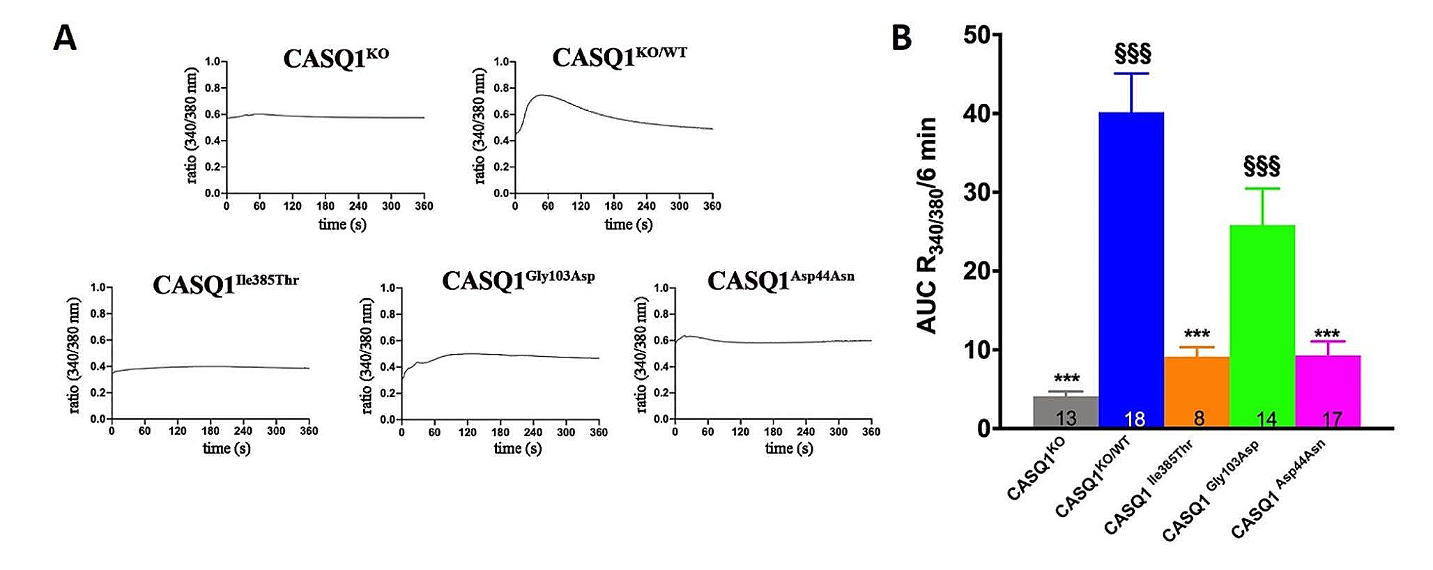
A two state kinetic scheme
Figure 1A illustrates a simple two-state kinetic scheme (Lymn and Taylor 1971; Goldman 1987; Cooke 1997; Sweeney et al. 2020) in which a myosin (M) motor with bound ADP (D) and inorganic phosphate (Pi) undergoes a switch-like lever arm rotation induced by actin (A) binding and gated by Pi release (MDP to AMD) (Huxley and Simmons 1971; Rayment et al. 1993; Finer et al. 1994; Baker et al. 1998, 2002). This molecular switch reversibly displaces a compliant element external to the motor a distance, d, with force-dependent forward, f+, and reverse, f–, rates (Baker et al. 2002; Stewart et al. 2021; Baker 2022). An ensemble of molecular switches is an entropic system spring (Baker 2022, 2023c).
For an equilibrium mixture of N parallel force generators, the displacement of a system spring by a single working step is d/N (displacing a single bed spring a distance, d, displaces the system of N parallel springs a distance d/N). At equilibrium, the system force, F, is distributed among all N myosin motors (Baker and Thomas 2000) because all motors (bound and detached) are inextricably part of and equilibrate with the macromolecular assembly to which force is applied. If only a fraction, a, of motors are equilibrated with the system force, the step size is d/(a·N), where the ergodic factor, a, ranges from 1 at an ergodic equilibrium to 1/N when on average only 1 of N motors is equilibrated with the system force.
Binding free energy
The Gibbs reaction free energy for actin-myosin binding (Fig. 1A) defined at a constant muscle force, F (Baker et al. 1999; Baker and Thomas 2000) is
$$_}\text = \varDelta }^} + \text\text\cdot\text\text\left[\right(_ + 1)/_]\hspace+\hspaceF\cdot$$
(1)
where ∆Go is the standard free energy for the binding reaction in Fig. 1A; NAMD and NMDP are the number of myosin motors in the AMD and MDP states (the total number of myosin motors is N = NAMD + NMDP); and the logarithmic term is the change in system entropy with a chemical step from to along the system reaction coordinate (Fig. 1C, y-axis, right to left) (Baker 2022). Here, I approximate (NAMD + 1) as NAMD and assume that fixed concentrations of actin and basal inorganic phosphate, Pi, are implicit in ∆Go.
An Entropic System Spring
Here I assume a thermodynamic force exerted on an entropic system spring (Fig. 1B, right side) defines the effective stiffness, κsys, of this spring (Baker 2022). I assume that one end of the spring (Fig. 1B, right) defines the macroscopic mechanical state of muscle (force, F, and length, L), while the other end of the spring (Fig. 1B, left) is stretched by force-generating switches that generate force in the spring through κsys⋅d/(aN) incremental displacements. In isometric muscle (the right side of the spring in Fig. 1B is fixed) no energy is lost to the surroundings as shortening heat or work, and so I refer to isometric force generation as adiabatic. In this case force, F, increases linearly with the number of bound myosin motors, NAMD, or decreases linearly with the number of detached myosin motors, NMDP, as
$$F = \kappa_\cdot/\left(aN\right)[_ - _^}}]$$
(2)
where NMDPo is NMDP at F = 0. Multiplying both sides of Eq. 2 by d/N
$$Fd/N = -a\left(_\cdot^\right)[_ - _^}}].$$
(3)
Equation 3 is plotted as Fd/N versus NMDP in Fig. 1C (solid black lines at NMDPo increments of 5).
Adiabatic (isometric) molecular force generation (Eq. 2) in the system spring continues until the force, F, reaches an isotherm (Eq. 1), which occurs when
$$Fd/N = a[\varDelta }^} + \text\text\cdot\text\text(_/_\left)\right].$$
(4)
The isotherm is ergodic if a = 1 and is otherwise non-ergodic. Equation 4 is plotted as Fd/N versus NMDP in Fig. 1C (colored curves with ∆Go increments of 1 kT).
Equations 3 and 4 are two different definitions of system force, F, distinguished by whether changes in muscle force occur adiabatically (Fig. 1C, left side) or isothermally (Fig. 1C, right side). In an ideal system (adiabatic or isothermal) the binding reaction follows one or the other of these pathways (black lines or colored curves in Fig. 1C). However in general these two processes can occur together, requiring that Eqs. 3 and 4 are coupled. The physical basis for this coupling are kinetic rates that are defined by the energetics in Eq. 4 as
$$_/f_ = \text\text\text\left[\right(-Fd/aN - \text\text\cdot\text\text(_/_) - \varDelta }^})/\text\text],$$
(5)
where Eq. 5 is simply the right-hand side of Eq. 1 rewritten to describe the probability of the muscle system being found in state relative to along a system reaction energy landscape that is tilted by the energy terms in Eq. 5 (Baker 2023c).
When a = 1, molecular force generation stalls along the ergodic isotherm (∆rG = 0) at a force, Fo = –N∆Go/d – NkT⋅ln(NAMD/NMDP). When a < 1, molecular force generation stalls along a non-ergodic (∆rG < 0) isotherm at a force, F = a⋅Fo. In general, non-ergodicity occurs when not all of the N myosin motors equilibrate with the system force. There are many possible mechanisms for non-ergodicity, including sequestration of myosin motors in inactive states, a stiff system that generates large forces with a small number of steps, and internal system forces that contribute to the total force with which motors equilibrate.
If the internal energy of a system is perturbed by δE, the system energy landscape is further tilted by δE along the system reaction coordinate (Baker 2023c), perturbing the kinetics of force generation from Eq. 5 as
$$_/_= \text\text\text\left[\right(-Fd/aN - \text\text\cdot\text\text(_/_) - \varDelta }^} - E)/\text\text].$$
(6)
For each energy term, E, in Eq. 6 the E-dependence of exp(E/kT) can be partitioned between forward, f+(E), and reverse, f–(E), rate constants through a coefficient, αE, that describes the fractional change in E prior to the activation energy barrier (Hille 1987). For example, when δE and F in Eq. 6 are zero,
$$_^} =_\, \text\text\text(-_\cdot\varDelta }^}/\text\text) \,and$$
$$_^} = _ \,\text\text\text\left[\right(1 - _)\varDelta }^}/\text\text)$$
are unloaded equilibrium rates.
The time courses for all processes, both ideal (Eqs. 3 and 4) and non-ideal (Eqs. 3 and 4 coupled through Eq. 6), are described by three simple master equations. The rate of the two-state reaction in Fig. 1A is
$$\text_/\text\text= -_ \cdot_ + _\cdot_,$$
(7)
which according to Eq. 2 generates force in the system spring at a rate
$$\textF/\text\text = (\text_/\text\text)\cdot_\cdot/N.$$
(8)
If force generation through Eq. 8 stalls at a non-ergodic isotherm, the system subsequently approaches an ergodic isotherm at a rate b (i.e., the rate at which a approaches 1), defining the third master Eq.
$$\text(1-a)/\text\text = -(1-a)b.$$
(9)
For each non-ergodic factor that “damps” or “frustrates” equilibration (e.g., a < 1), there is a corresponding process (with a unique rate, b) through which the system reaches an ergodic equilibrium. This need not be a single exponential process. If b = 0, muscle is stuck in a state (e.g., smooth muscle latch) analogous to a frustrated spin state (Baker et al. 2003).
From these equations (Eqs. 7–9), four phases of a force transient are evident. The initial perturbation, δE, from equilibrium is phase (1) Force generation that reaches a non-ergodic isotherm (Eq. 8) is phase (2) Chemical relaxation toward the ergodic isotherm (Eq. 9) is phase (3) And a return to the original stall force along the equilibrium isotherm is phase (4) All simulations below are based on these three master equations (Eqs. 7–9) with rate constants defined from first principles (Eq. 6) and parameters defined in Table 1.
Thermodynamic analysis
Equation 3 (black lines) and 4 (colored curves) are plotted in Fig. 1C. Equation 4 is plotted at different ∆Go values (1 kT increments), and Eq. 3 is plotted at different NMo values (increments of 5). Each line represents a reversible binding reaction, and many complex mechanical behaviors resembling muscle mechanics emerge from these binding pathways.
Computer simulations
Using master Eqs. 7, 8 and 9, the rate constants defined by Eq. 6, and model parameters in Table 1, MatLab (Mathworks, Natick, MA) is used to simulate muscle force transients.


Comments (0)