Study species and housing

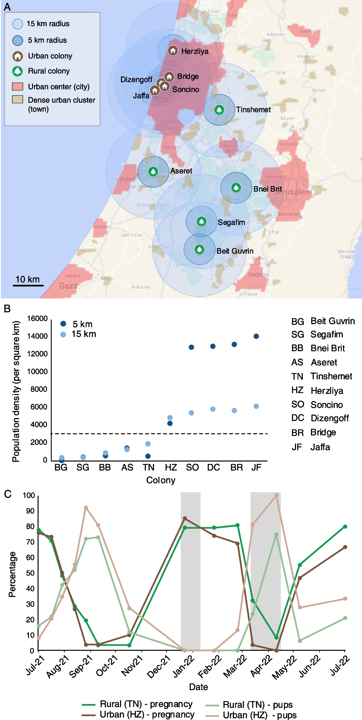
The study comprised 25 Egyptian fruit bats (Rousettus aegyptiacus) (12 females: 8 adults, 4 juveniles; and 13 males: 11 adults, 2 juveniles, see Table 2). The adult bats were captured in a natural colony in central Israel (Herzliya) in December 2019 and were housed together with an already existing colony of Egyptian fruit bats. The juvenile bats were either born in our captive colony or brought to the colony with their mothers at a very early age.

Table 2 The 25 bats that participated in the study. Asterisks mark bats that were born in the captive colony. The table indicates which environmental condition was experienced by each bat

The colony (4 × 2 × 2.9 m3) comprised a total of 30 bats. They were kept under a 12:12 light to dark cycle, at a stable temperature of 24 ± 2 °C.

Experimental setup

The experiments took place in two identical tents (2.4 × 2.4 × 1.85 m3) in a controlled temperature room (24 ± 2 °C), next to the captive bats’ colony, allowing the bats in the tents to hear the sounds from the colony and thereby reduce stress. The floor underneath each tent was covered with 25 pieces of 50 × 50 × 1 cm soft foam mat, to prevent bat injury in case of a fall. The tent walls were covered with black felt from about 1 m above the floor to the tent top, allowing the bats to hang anywhere. A 30 × 30 cm2 plastic net was placed at the top of the tent to enable perching. Each tent held two feeders, placed one meter apart. Each feeder (see Fig. 2A) contained a 50 × 50 × 1 cm3 vertical wooden platform covered with felt and a plastic net. A pump was installed on the side of the wooden square, with a 5-mm pipe that ended in a 10-ml tube. Another pipe was connected to the tube, allowing a max of 6 ml of juice to accumulate in the tube. The pumps were programmed to secret 3 ml of mango juice whenever a bat landed on the platform. Detection of landing was based on RFID. All landings were logged to a computer. A GeoVision camera located on the floor filmed the two feeders during the experiments.

Fig. 2

A Experimental setup. (a) Two feeders with landing platforms and RFID antennas. (b) A—juice pump, B—feeding tube, C—RFID antenna. The bottle on the side collected juice spillover, allowing us to quantify drinking. B The experimental procedure—phase 1: both of the feeders reward with p(reward) = 1. Phase 2: the bats were divided between a stable and a volatile environment. The rewarding feeder (p(reward) = 0.8) and the less rewarding feeder (p(reward) = 0.2) changed either every hour (volatile environment) or after 2 nights (stable environment)

Experimental procedure

The experiments consisted of two phases: the exposure phase and the learning phase (see Fig. 2B). All experiments took place at night, the bats’ natural activity time, from around 16:00 to around 9:00 the next day, after the same number of hours since being fed. The bats were kept in the captive colony in between experiments. In addition to the mango-juice feeders, a bowl of water was permanently available in the tents.

Phase 1: Exposure

The goal of this phase was to familiarize the bats with the experimental setting and to ensure that they had learned to feed from the feeders. To reduce the bats’ stress, the exposure phase was done using pairs of bats. The bats were kept in the experimental tent for one night and both feeders provided a reward of 3 ml of mango juice for each landing.

Phase 2: Learning

In this phase, we measured the bats’ learning rate. Each bat was kept alone in the same experiment tent for four consecutive nights. One of the feeders was more rewarding (hereafter the “rewarding feeder”) with a probability of 0.8 of providing a reward with each landing, while the other feeder was less rewarding (hereafter the “less rewarding feeder”), with a probability of only 0.2 of providing a reward. The first position of the rewarding feeder was on the right side of the tent for half of the bats and on the left for the other half. The bats were randomly allocated to either a stable or a volatile environment. In the stable environment, the rewarding and the less rewarding feeders remained in the same positions for two consecutive nights, after which their positions were switched. In the volatile environment, the position switch between the rewarding and the less rewarding feeders was systematically applied every hour (i.e., R-L-R-L).

Fifteen bats (10 adults and 5 juveniles) were exposed to a stable environment, and 10 bats were exposed to a volatile environment. During the daytime, the bats were returned to their colony.

Analysis

A trial was defined as a bat landing on a feeder—either when switching from one feeder to the other or when landing on the same feeder, when at least three seconds had passed from the time of previously leaving that feeder. We extracted the following information for each bat: the time of each landing, the chosen feeder in each trial, the reward the bat received (0 for no reward or 1 if it received a reward) in each trial, and the total number of trials.

Estimating the bats’ learning rates- Reinforcement-learning models

We tested two models—a model without choice perseveration and a model with choice perseveration, as explained below, using MATLAB scripts.

We used maximum-likelihood estimation using the Matlab function “optimoptions” to estimate bats’ individual parameters. For each bat, we used 50 starting points that were randomly chosen by the computer. We used the best fitting parameters as an estimate for the bats' latent learning parameters. We compared the models’ fit using a BIC score.

Model without perseveration

We used a Q-learning model to calculate the learning rate (α). We simulated Q-values for each action on each step and the probability of choosing each action according to the SoftMax policy (see Eq. 1) [15, 23], where β is the inverse temperature parameter, i.e., the parameter that determines the sensitivity of the choice probabilities to the difference in values. Large values of β make the choice more sensitive to the values difference, while low values of β make the choice less sensitive to the difference in values [15, 23].

$$P\left(a\left(t\right)=1\right)=\frac_) }(\beta _) +exp(\beta _)}$$

(1)

where \(_\) is the Q-value for the chosen action i (a or b), β is the inverse temperature parameter, and t is the index of the trial.

Q-values are updated based on the outcome (see Eq. 2).

$$_(t+1)=_(t)+\alpha *(Reward(t)-_(t))$$

(2)

where \(_\) is the Q-value for the chosen action i, and t is the index of the trial. α is the learning rate. The Q-value of the unchosen action is not updated [15].

Model with choice perseveration

The model with perseveration includes a learning rate (α) and inverse temperature (β) as in the model without perseveration, together with two additional parameters that represent the bats’ perseveration behavior (the perseveration rate and perseveration exponent). This model keeps track of choice perseveration values (\(_\)) for each action, which determines the perseveration strengths of each action (similar in spirit to the Q-values). The \(_\) are initiated at 0.5 and updated after each trial according to the perseveration rate (\(_\)) free parameter (between 0 and 1), which determines the magnitude of updating. The updating increases the \(_\) of the selected action toward 1 and the unselected action \(_\) toward 0, regardless of the outcome (see Eq. 3). We also included an additional perseveration exponent (\(_\)) free parameter which determines how perseverative the bat is; note that the setting \(_=0\) is exactly like the RL model without perseveration. Q-values are updated similarly to the model without perseveration (see Eq. 2) [19, 20].

$$\beginp\left(a\left(t\right)=1\right)=\frac(\upbeta *_+_*_)}\left(\upbeta *_+_*_\right)+\mathrm\left(\beta *_+_*_\right)}\\ _=\left(1-_}\right)* _\\ \begin_=\left(1-_}\right)*_\\ _\right)}=_\right)}+_\end\end$$

(3)

where a is the action, β is the inverse temperature parameter, \(_\) is the Q value for the chosen action i (a or b), P exp is the perseveration exponent, P val is perseveration value, and t is the index of the trial).

Reward effect on stay probability

Staying was defined as returning to the feeder that had been visited in the previous trial. We estimated the stay probabilities (for each individual) in both the cases in which the bat had received a reward in the previous trial and in which it had not. To examine the effect of reward on the stay probability (which we term the “reward effect”), we subtracted the individual stay probability for no reward from that following reward (see Eq. 4).

$$\mathrm\;\mathrm=P\left(\mathrm\vert\mathrm\right)-P\left(\mathrm\vert\mathrm\;\mathrm\right)$$

(4)

Foraging efficiency

To determine bats’ foraging efficiency, we calculated their success rate. Success rate was defined as the proportion of actions that led to reward (see Eq. 5).

$$\mathrm\;\mathrm=\frac\;\mathrm\;\mathrm\;\mathrm}\;\mathrm}$$

(5)

Reinforcement-learning simulations

To examine whether the bats employed an optimal learning rate that would maximize their success rate, we simulated data using a grid search separately for each environment and noted the resulting success rates. Specifically, we changed the learning rate gradually from 0 to 1 in steps of 0.1. For each learning rate value in the grid search, each agent was simulated using a β parameter that was sampled from the empirical β distribution estimated for the bats (i.e., the bats’ estimated β were used), separately for each environment. Since in the stable environment there were 13 bats each tested for four nights, and one bat that was tested for only two nights, this totaled on 54 bats’ estimated β. Each estimated β was used twice, thus simulating 108 agents in total in the stable environment for each learning rate. In the volatile environment, nine bats had been tested each for four nights, resulting in 36 estimated β. Each estimated β was used by three agents, thus simulating 108 agents in total in the volatile environment for each learning rate. The number of trials was 2000 in each simulation.

In our empirical setting, the stable group had a fixed reward probability for each feeder for two nights and a reversed probability for two additional nights; while the volatile group received reversal in the reward probability every hour. Bats in the stable environment performed on average 251 trials on nights 1–2 before the reversal in probability and 214 trials on nights 3–4 (after the reversal in probability). Thus, for the stable environment simulation, we used the same fixed reward probability as in our empirical settings for 251 trials, then switched the reward probability between the choices for 214 trials and returned this process until 2000 trials had been carried out. For the volatile environment, we switched the reward probability every 13 trials until reaching 2000 trials. This was done because in the volatile environment the bats had performed 13 trials on average within an hour, before the reward probabilities were switched. The simulations are equivalent to the no perseveration model without an adjustment of the Q-values between ‘nights’; i.e., we did not simulate forgetting.

Win-Stay-Lose-Shift (WSLS) model

Given the binary decision of the task, we modeled a WSLS rule-based strategy [24, 25]. Allowing for some deviation from the deterministic ruling, we used a two free parameter model—the Win-Stay probability (\(_)\), which is the probability that the bat returns to the same feeder in the next trial after receiving a reward from it in the previous trial, and the Lose-Shift probability (\(_)\), which is the probability that the bat shifts to the other feeder in the next trial after not receiving a reward from it in the previous trial (see Eq. 6).

$$p\left(a(t)=i\right)= \left\_ \\ _ \end\right.\begin\mathrm\\ \mathrm\end\begin_=_\mathrm\;\;_=1 \\ _=_\mathrm\;\;_=0\end$$

(6)

The probability of choosing action i if action i had been chosen in the previous trial is either \(_\) or \(_\), depending on the previous reward. a is the action, t is the index of the trial, and r is the reward (1 or 0).

Parameter estimation for each bat’s decisions was done using maximum-likelihood with a self-written Python script.

WSLS simulations

For each environment (e.g., stable or volatile) and for each combination of WSLS model parameters (from 0 to 1 in steps of 0.1), we ran 100 simulations of 2000 trials each. The reward probability of each action was identical to those used in the real bat experiments. We averaged across the 100 simulations of each environment and parameter combination and calculated the success rate (Eq. 5).

Discarded data

Due to a mechanical problem in the feeding system, one of the bats (bat 18, the stable environment group) did not obtain any rewards during its third night in the experiment. Data from the third and fourth nights of this bat were therefore discarded. When examining the effect of reward on the stay probability, two bats (bat 1, stable environment group; and bat 8, volatile environment group) demonstrated a negative effect in three out of the four experimental nights. This suggests that they had failed to learn, and they were consequently also removed from the analysis.

Statistics

We used a mixed-effects generalized linear model—GLMM—with α—the learning rate set as the explanatory parameter, the environment and night as fixed effects, and subject ID as a random effect. To examine the effect of the environment (stable vs. volatile) on the learning rate, the model without the sex interaction produced a better fit (BIC =  − 8.08 for the model without sex interaction vs BIC =  − 7.05 for the model with sex interaction). To determine the effect of the environment on success rate, we used a GLMM, with the success rate set as the explanatory parameter, with a logit link function, and the other parameters as above. To determine the significance of the reward effect on stay probability, we used a one-sample one-sided T-test on each group (stable or volatile). To determine the nightly reward effect on stay probability, we used Pearson’s correlation of median reward effect with night number (1–4).

To determine the difference in success rate between the real bats and the simulations, we compared the real bats’ success rate to 108 reinforcement-learning simulations (with optimal alpha) and to 100 WSLS simulations with the same parameters as estimated for the bats and examined whether the bats’ success rate in each group was in the lowest or highest 5% of the simulations’ success rate within the same environment.

To compare between all the reinforcement models, we used BIC. BIC is considered to be more conservative than AIC and therefore more suitable for a small sample size in estimating model fit.

To compare between the reinforcement-learning model without choice perseveration and the Win-Stay-Lose-Shift model, we compared their log-likelihoods, since both models have the same number of free parameters. All the results are presented as mean ± SD.